Chapter 13: Statistics - Pre-pre-school

Chapter 13: Statistics

Robert Johansson

Source code listings for Numerical Python - Scientific Computing and Data Science Applications with Numpy, SciPy and Matplotlib (ISBN 979-8-8688-0412-0).

Imports¶

from scipy import stats

from scipy import optimize

import random

import numpy as np

%matplotlib inline
import matplotlib.pyplot as plt

import matplotlib as mpl

mpl.rcParams["mathtext.fontset"] = "stix"
mpl.rcParams["font.family"] = "serif"
mpl.rcParams["font.sans-serif"] = "stix"

import seaborn as sns

sns.set(style="whitegrid")

Descriptive statistics¶

x = np.array([3.5, 1.1, 3.2, 2.8, 6.7, 4.4, 0.9, 2.2])

np.mean(x)

np.float64(3.1)

np.median(x)

np.float64(3.0)

x.min(), x.max()

(np.float64(0.9), np.float64(6.7))

x.var()

np.float64(3.0700000000000007)

x.std()

np.float64(1.7521415467935233)

x.var(ddof=1)

np.float64(3.5085714285714293)

x.std(ddof=1)

np.float64(1.8731181032095732)

Random numbers¶

random.seed(123456789)

random.random()

0.6414006161858726

random.randint(0, 10)  # 0 and 10 inclusive

8

np.random.seed(123456789)

np.random.rand()

0.532833024789759

np.random.randn()

0.8768342101492541

np.random.rand(5)

array([0.71356403, 0.25699895, 0.75269361, 0.88387918, 0.15489908])

np.random.randn(2, 4)

array([[ 3.13325952,  1.15727052,  1.37591514,  0.94302846],
       [ 0.8478706 ,  0.52969142, -0.56940469,  0.83180456]])

np.random.randint(10, size=10)

array([0, 3, 8, 3, 9, 0, 6, 9, 2, 7])

np.random.randint(low=10, high=20, size=(2, 10))

array([[12, 18, 18, 17, 14, 12, 14, 10, 16, 19],
       [15, 13, 15, 18, 11, 17, 17, 10, 13, 17]])

fig, axes = plt.subplots(1, 3, figsize=(12, 3))

axes[0].hist(np.random.rand(10000))
axes[0].set_title("rand")
axes[1].hist(np.random.randn(10000))
axes[1].set_title("randn")
axes[2].hist(np.random.randint(low=1, high=10, size=10000), bins=9, align="left")
axes[2].set_title("randint(low=1, high=10)")

fig.tight_layout()
fig.savefig("ch13-random-hist.pdf")

# random.sample(range(10), 5)

np.random.choice(10, 5, replace=False)

array([9, 0, 5, 8, 1])

np.random.seed(123456789)

np.random.rand()

0.532833024789759

np.random.seed(123456789)
np.random.rand()

0.532833024789759

np.random.seed(123456789)
np.random.rand()

0.532833024789759

prng = np.random.RandomState(123456789)

prng.randn(2, 4)

array([[ 2.212902  ,  2.1283978 ,  1.8417114 ,  0.08238248],
       [ 0.85896368, -0.82601643,  1.15727052,  1.37591514]])

prng.chisquare(1, size=(2, 2))

array([[1.26859720e+00, 2.02731988e+00],
       [2.52605129e-05, 3.00376585e-04]])

prng.standard_t(1, size=(2, 3))

array([[ 0.59734384, -1.27669959,  0.09724793],
       [ 0.22451466,  0.39697518, -0.19469463]])

prng.f(5, 2, size=(2, 4))

array([[ 0.77372119,  0.1213796 ,  1.64779052,  1.21399831],
       [ 0.45471421, 17.64891848,  1.48620557,  2.55433261]])

prng.binomial(10, 0.5, size=10)

array([8, 3, 4, 2, 4, 5, 4, 4, 7, 5])

prng.poisson(5, size=10)

array([7, 1, 3, 4, 6, 4, 9, 7, 3, 6])

Probability distributions and random variables¶

np.random.seed(123456789)

X = stats.norm(1, 0.5)

X.mean()

np.float64(1.0)

X.median()

np.float64(1.0)

X.std()

np.float64(0.5)

X.var()

np.float64(0.25)

[X.moment(n) for n in range(5)]

[np.float64(1.0),
 np.float64(1.0),
 np.float64(1.25),
 np.float64(1.75),
 np.float64(2.6875)]

X.stats()

(np.float64(1.0), np.float64(0.25))

X.pdf([0, 1, 2])

array([0.10798193, 0.79788456, 0.10798193])

X.cdf([0, 1, 2])

array([0.02275013, 0.5 , 0.97724987])

X.rvs(10)

array([2.106451  , 2.0641989 , 1.9208557 , 1.04119124, 1.42948184,
       0.58699179, 1.57863526, 1.68795757, 1.47151423, 1.4239353 ])

stats.norm(1, 0.5).stats()

(np.float64(1.0), np.float64(0.25))

stats.norm.stats(loc=2, scale=0.5)

(np.float64(2.0), np.float64(0.25))

X.interval(0.95)

(np.float64(0.020018007729972975), np.float64(1.979981992270027))

X.interval(0.99)

(np.float64(-0.2879146517744502), np.float64(2.28791465177445))

def plot_rv_distribution(X, axes=None):
    """Plot the PDF, CDF, SF and PPF of a given random variable"""
    if axes is None:
        fig, axes = plt.subplots(1, 3, figsize=(12, 3))

    x_min_999, x_max_999 = X.interval(0.999)
    x999 = np.linspace(x_min_999, x_max_999, 1000)

    x_min_95, x_max_95 = X.interval(0.95)
    x95 = np.linspace(x_min_95, x_max_95, 1000)

    if hasattr(X.dist, "pdf"):
        axes[0].plot(x999, X.pdf(x999), label="PDF")
        axes[0].fill_between(x95, X.pdf(x95), alpha=0.25)
    else:
        x999_int = np.unique(x999.astype(int))
        axes[0].bar(x999_int, X.pmf(x999_int), label="PMF")
    axes[1].plot(x999, X.cdf(x999), label="CDF")
    axes[1].plot(x999, X.sf(x999), label="SF")
    axes[2].plot(x999, X.ppf(x999), label="PPF")

    for ax in axes:
        ax.legend()

    return axes

fig, axes = plt.subplots(3, 3, figsize=(12, 9))

X = stats.norm()
plot_rv_distribution(X, axes=axes[0, :])
axes[0, 0].set_ylabel("Normal dist.")
X = stats.f(2, 50)
plot_rv_distribution(X, axes=axes[1, :])
axes[1, 0].set_ylabel("F dist.")
X = stats.poisson(5)
plot_rv_distribution(X, axes=axes[2, :])
axes[2, 0].set_ylabel("Poisson dist.")

fig.tight_layout()
fig.savefig("ch13-distributions.pdf")

def plot_dist_samples(X, X_samples, title=None, ax=None):
    """Plot the PDF and histogram of samples of a continuous random variable"""
    if ax is None:
        fig, ax = plt.subplots(1, 1, figsize=(8, 4))

    x_lim = X.interval(0.99)
    x = np.linspace(*x_lim, num=100)

    ax.plot(x, X.pdf(x), label="PDF", lw=3)
    ax.hist(X_samples, label="samples", density=True, bins=75)
    ax.set_xlim(*x_lim)
    ax.legend()

    if title:
        ax.set_title(title)
    return ax

fig, axes = plt.subplots(1, 3, figsize=(12, 3))
X = stats.t(7.0)
plot_dist_samples(X, X.rvs(2000), "Student's t dist.", ax=axes[0])
X = stats.chi2(5.0)
plot_dist_samples(X, X.rvs(2000), r"$\chi^2$ dist.", ax=axes[1])
X = stats.expon(0.5)
plot_dist_samples(X, X.rvs(2000), "exponential dist.", ax=axes[2])
fig.tight_layout()
fig.savefig("ch13-dist-sample.pdf")

X = stats.chi2(df=5)

X_samples = X.rvs(500)

df, loc, scale = stats.chi2.fit(X_samples)

df, loc, scale

(np.float64(4.728645123391404),
 np.float64(0.03257330219133387),
 np.float64(1.0734482977974253))

Y = stats.chi2(df=df, loc=loc, scale=scale)

fig, ax = plt.subplots(1, 1, figsize=(8, 3))

x_lim = X.interval(0.99)
x = np.linspace(*x_lim, num=100)

ax.plot(x, X.pdf(x), label="original")
ax.plot(x, Y.pdf(x), label="recreated")
ax.legend()

fig.tight_layout()
fig.savefig("ch13-max-likelihood-fit.pdf")

fig, axes = plt.subplots(1, 2, figsize=(12, 4))

x_lim = X.interval(0.99)
x = np.linspace(*x_lim, num=100)

axes[0].plot(x, X.pdf(x), label="original")
axes[0].plot(x, Y.pdf(x), label="recreated")
axes[0].legend()

axes[1].plot(x, X.pdf(x) - Y.pdf(x), label="error")
axes[1].legend()

fig.tight_layout()
fig.savefig("ch13-max-likelihood-fit.pdf")

Hypothesis testing¶

np.random.seed(123456789)

mu, sigma = 1.0, 0.5

X = stats.norm(mu - 0.2, sigma)

n = 100

X_samples = X.rvs(n)

z = (X_samples.mean() - mu) / (sigma / np.sqrt(n))

np.float64(-2.8338979550098298)

t = (X_samples.mean() - mu) / (X_samples.std(ddof=1) / np.sqrt(n))

np.float64(-2.9680338545657845)

stats.norm().ppf(0.025)

np.float64(-1.9599639845400545)

2 * stats.norm().cdf(-abs(z))

np.float64(0.004598401329075357)

2 * stats.t(df=(n - 1)).cdf(-abs(t))

np.float64(0.003758647967422724)

t, p = stats.ttest_1samp(X_samples, mu)

np.float64(-2.968033854565784)

np.float64(0.003758647967422724)

fig, ax = plt.subplots(figsize=(8, 3))

sns.histplot(X_samples, ax=ax, kde=True, stat="density")
x = np.linspace(*X.interval(0.999), num=100)
ax.plot(x, stats.norm(loc=mu, scale=sigma).pdf(x))

fig.tight_layout()
fig.savefig("ch13-hypothesis-test-dist-sample-mean.pdf")

n = 50

mu1, mu2 = np.random.rand(2)

mu1, mu2

(np.float64(0.24764580637159606), np.float64(0.42145435527527897))

X1 = stats.norm(mu1, sigma)

X1_sample = X1.rvs(n)

X2 = stats.norm(mu2, sigma)

X2_sample = X2.rvs(n)

t, p = stats.ttest_ind(X1_sample, X2_sample)

np.float64(-1.4283175246005888)

np.float64(0.1563798105967323)

mu1, mu2

(np.float64(0.24764580637159606), np.float64(0.42145435527527897))

sns.histplot(X1_sample)
sns.histplot(X2_sample)

<Axes: ylabel='Count'>

Nonparameteric methods¶

np.random.seed(0)

X = stats.chi2(df=5)

X_samples = X.rvs(100)

kde = stats.gaussian_kde(X_samples)

kde_low_bw = stats.gaussian_kde(X_samples, bw_method=0.25)

x = np.linspace(0, 20, 100)

fig, axes = plt.subplots(1, 3, figsize=(12, 3))

axes[0].hist(X_samples, density=True, alpha=0.5, bins=25)
axes[1].plot(x, kde(x), label="KDE")
axes[1].plot(x, kde_low_bw(x), label="KDE (low bw)")
axes[1].plot(x, X.pdf(x), label="True PDF")
axes[1].legend()
sns.histplot(X_samples, bins=25, ax=axes[2], kde=True, stat="density")

fig.tight_layout()
fig.savefig("ch13-hist-kde.pdf")

kde.resample(10)

array([[ 1.10979087,  0.4379679 , 14.20879078,  5.94683846,  1.78490438,
         5.58416739,  4.18349885,  2.78527976,  0.68112826,  7.7643985 ]])

def _kde_cdf(x):
    return kde.integrate_box_1d(-np.inf, x)

kde_cdf = np.vectorize(_kde_cdf)

fig, ax = plt.subplots(1, 1, figsize=(8, 3))

sns.histplot(X_samples, bins=25, ax=ax, kde=True, stat="density")
x = np.linspace(0, 20, 100)
ax.plot(x, kde_cdf(x))

fig.tight_layout()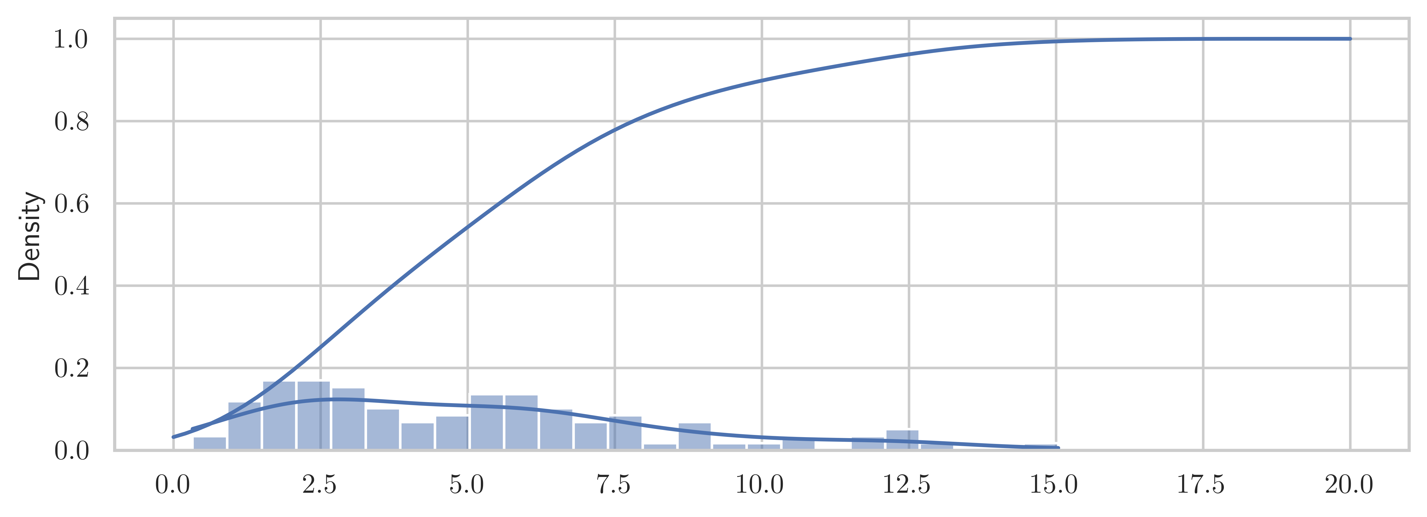

def _kde_ppf(q):
    return optimize.fsolve(lambda x, q: kde_cdf(x) - q, kde.dataset.mean(), args=(q,))[
        0
    ]

kde_ppf = np.vectorize(_kde_ppf)

kde_ppf([0.05, 0.95])

array([ 0.39074674, 11.94993578])

X.ppf([0.05, 0.95])

array([ 1.14547623, 11.07049769])

References¶

Johansson, R. (2024). Numerical Python: Scientific Computing and Data Science Applications with Numpy, SciPy and Matplotlib. Apress. 10.1007/979-8-8688-0413-7