Chapter 12: Data processing and analysis with pandas
Robert Johansson
Source code listings for Numerical Python - Scientific Computing and Data Science Applications with Numpy, SciPy and Matplotlib (ISBN 979-8-8688-0412-0).
%matplotlib inline
import matplotlib.pyplot as plt
import numpy as npimport pandas as pd# pd.set_option('display.mpl_style', 'default')import matplotlib as mpl
mpl.style.use("ggplot")import seaborn as snsSeries object
s = pd.Series([909976, 8615246, 2872086, 2273305])s0 909976
1 8615246
2 2872086
3 2273305
dtype: int64type(s)pandas.core.series.Seriess.dtypedtype('int64')s.indexRangeIndex(start=0, stop=4, step=1)s.valuesarray([ 909976, 8615246, 2872086, 2273305])s.index = ["Stockholm", "London", "Rome", "Paris"]s.name = "Population"sStockholm 909976
London 8615246
Rome 2872086
Paris 2273305
Name: Population, dtype: int64s = pd.Series(
[909976, 8615246, 2872086, 2273305],
index=["Stockholm", "London", "Rome", "Paris"],
name="Population",
)s["London"]np.int64(8615246)s.Stockholmnp.int64(909976)s[["Paris", "Rome"]]Paris 2273305
Rome 2872086
Name: Population, dtype: int64s.median(), s.mean(), s.std()(np.float64(2572695.5), np.float64(3667653.25), np.float64(3399048.5005155364))s.min(), s.max()(np.int64(909976), np.int64(8615246))s.quantile(q=0.25), s.quantile(q=0.5), s.quantile(q=0.75)(np.float64(1932472.75), np.float64(2572695.5), np.float64(4307876.0))s.describe()count 4.000000e+00
mean 3.667653e+06
std 3.399049e+06
min 9.099760e+05
25% 1.932473e+06
50% 2.572696e+06
75% 4.307876e+06
max 8.615246e+06
Name: Population, dtype: float64fig, axes = plt.subplots(1, 4, figsize=(12, 3.5))
s.plot(ax=axes[0], kind="line", title="line")
s.plot(ax=axes[1], kind="bar", title="bar")
s.plot(ax=axes[2], kind="box", title="box")
s.plot(ax=axes[3], kind="pie", title="pie")
fig.tight_layout()
fig.savefig("ch12-series-plot.pdf")
fig.savefig("ch12-series-plot.png")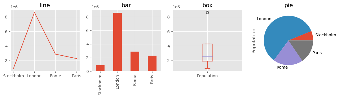
DataFrame object
df = pd.DataFrame(
    [
        [909976, 8615246, 2872086, 2273305],
        ["Sweden", "United kingdom", "Italy", "France"],
    ]
)dfLoading...
df = pd.DataFrame(
    [
        [909976, "Sweden"],
        [8615246, "United kingdom"],
        [2872086, "Italy"],
        [2273305, "France"],
    ]
)dfLoading...
df.index = ["Stockholm", "London", "Rome", "Paris"]df.columns = ["Population", "State"]dfLoading...
df = pd.DataFrame(
    [
        [909976, "Sweden"],
        [8615246, "United kingdom"],
        [2872086, "Italy"],
        [2273305, "France"],
    ],
    index=["Stockholm", "London", "Rome", "Paris"],
    columns=["Population", "State"],
)dfLoading...
df = pd.DataFrame(
    {
        "Population": [909976, 8615246, 2872086, 2273305],
        "State": ["Sweden", "United kingdom", "Italy", "France"],
    },
    index=["Stockholm", "London", "Rome", "Paris"],
)dfLoading...
df.indexIndex(['Stockholm', 'London', 'Rome', 'Paris'], dtype='object')df.columnsIndex(['Population', 'State'], dtype='object')df.valuesarray([[909976, 'Sweden'],
[8615246, 'United kingdom'],
[2872086, 'Italy'],
[2273305, 'France']], dtype=object)df.PopulationStockholm 909976
London 8615246
Rome 2872086
Paris 2273305
Name: Population, dtype: int64df["Population"]Stockholm 909976
London 8615246
Rome 2872086
Paris 2273305
Name: Population, dtype: int64type(df.Population)pandas.core.series.Seriesdf.Population.Stockholmnp.int64(909976)type(df.index)pandas.core.indexes.base.Indexdf.loc["Stockholm"]Population 909976
State Sweden
Name: Stockholm, dtype: objecttype(df.loc["Stockholm"])pandas.core.series.Seriesdf.loc[["Paris", "Rome"]]Loading...
df.loc[["Paris", "Rome"], "Population"]Paris 2273305
Rome 2872086
Name: Population, dtype: int64df.loc["Paris", "Population"]np.int64(2273305)df[["Population"]].mean()Population 3667653.25
dtype: float64df.info()<class 'pandas.core.frame.DataFrame'>
Index: 4 entries, Stockholm to Paris
Data columns (total 2 columns):
# Column Non-Null Count Dtype
--- ------ -------------- -----
0 Population 4 non-null int64
1 State 4 non-null object
dtypes: int64(1), object(1)
memory usage: 268.0+ bytes
df.dtypesPopulation int64
State object
dtype: objectdf.head()Loading...
!head -n5 european_cities.csvRank,City,State,Population,Date of census/estimate
1,London[2], United Kingdom,"8,615,246",1 June 2014
2,Berlin, Germany,"3,437,916",31 May 2014
3,Madrid, Spain,"3,165,235",1 January 2014
4,Rome, Italy,"2,872,086",30 September 2014
Larger dataset
df_pop = pd.read_csv("european_cities.csv")df_pop.head()Loading...
df_pop = pd.read_csv("european_cities.csv", delimiter=",", encoding="utf-8", header=0)df_pop.info()<class 'pandas.core.frame.DataFrame'>
RangeIndex: 105 entries, 0 to 104
Data columns (total 5 columns):
# Column Non-Null Count Dtype
--- ------ -------------- -----
0 Rank 105 non-null int64
1 City 105 non-null object
2 State 105 non-null object
3 Population 105 non-null object
4 Date of census/estimate 105 non-null object
dtypes: int64(1), object(4)
memory usage: 4.2+ KB
df_pop.head()Loading...
df_pop["NumericPopulation"] = df_pop.Population.apply(lambda x: int(x.replace(",", "")))df_pop["State"].values[:3]array([' United Kingdom', ' Germany', ' Spain'], dtype=object)df_pop["State"] = df_pop["State"].apply(lambda x: x.strip())df_pop.head()Loading...
df_pop.dtypesRank int64
City object
State object
Population object
Date of census/estimate object
NumericPopulation int64
dtype: objectdf_pop2 = df_pop.set_index("City")df_pop2 = df_pop2.sort_index()df_pop2.head()Loading...
df_pop2.head()Loading...
df_pop3 = df_pop.set_index(["State", "City"]).sort_index(level=0)df_pop3.head(7)Loading...
df_pop3.loc["Sweden"]Loading...
df_pop3.loc[("Sweden", "Gothenburg")]Rank 53
Population 528,014
Date of census/estimate 31 March 2013
NumericPopulation 528014
Name: (Sweden, Gothenburg), dtype: objectdf_pop.set_index("City").sort_values(
["State", "NumericPopulation"], ascending=[False, True]
).head()Loading...
city_counts = df_pop.State.value_counts()city_counts.name = "# cities in top 105"df_pop3 = df_pop[["State", "City", "NumericPopulation"]].set_index(["State", "City"])
df_pop3Loading...
# df_pop3.sum(level="State")
# df_pop4 = df_pop3.sum(level="State").sort_values("NumericPopulation", ascending=False)
# df_pop4
df_pop4 = (
df_pop3.groupby(level="State")
.sum()
.sort_values("NumericPopulation", ascending=False)
)df_pop4.head()Loading...
df_popLoading...
df_pop5 = (
    df_pop[["State", "NumericPopulation"]]
    .groupby("State")
    .sum()
    .sort_values("NumericPopulation", ascending=False)
)
df_pop5 = (
df_pop.drop("Rank", axis=1) # [["State", "NumericPopulation"]]
.groupby("State")
.sum()
.sort_values("NumericPopulation", ascending=False)
)df_pop5.head()Loading...
fig, (ax1, ax2) = plt.subplots(1, 2, figsize=(12, 4))

city_counts.plot(kind="barh", ax=ax1)
ax1.set_xlabel("# cities in top 105")
df_pop5.NumericPopulation.plot(kind="barh", ax=ax2)
ax2.set_xlabel("Total pop. in top 105 cities")

fig.tight_layout()
fig.savefig("ch12-state-city-counts-sum.pdf")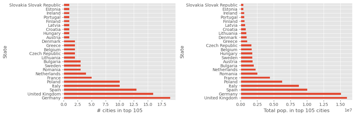
Time series
Basics
import datetimepd.date_range("2015-1-1", periods=31)DatetimeIndex(['2015-01-01', '2015-01-02', '2015-01-03', '2015-01-04',
'2015-01-05', '2015-01-06', '2015-01-07', '2015-01-08',
'2015-01-09', '2015-01-10', '2015-01-11', '2015-01-12',
'2015-01-13', '2015-01-14', '2015-01-15', '2015-01-16',
'2015-01-17', '2015-01-18', '2015-01-19', '2015-01-20',
'2015-01-21', '2015-01-22', '2015-01-23', '2015-01-24',
'2015-01-25', '2015-01-26', '2015-01-27', '2015-01-28',
'2015-01-29', '2015-01-30', '2015-01-31'],
dtype='datetime64[ns]', freq='D')pd.date_range(datetime.datetime(2015, 1, 1), periods=31)DatetimeIndex(['2015-01-01', '2015-01-02', '2015-01-03', '2015-01-04',
'2015-01-05', '2015-01-06', '2015-01-07', '2015-01-08',
'2015-01-09', '2015-01-10', '2015-01-11', '2015-01-12',
'2015-01-13', '2015-01-14', '2015-01-15', '2015-01-16',
'2015-01-17', '2015-01-18', '2015-01-19', '2015-01-20',
'2015-01-21', '2015-01-22', '2015-01-23', '2015-01-24',
'2015-01-25', '2015-01-26', '2015-01-27', '2015-01-28',
'2015-01-29', '2015-01-30', '2015-01-31'],
dtype='datetime64[ns]', freq='D')pd.date_range("2015-1-1 00:00", "2015-1-1 12:00", freq="H")/tmp/ipykernel_73526/4174652091.py:1: FutureWarning: 'H' is deprecated and will be removed in a future version, please use 'h' instead.
pd.date_range("2015-1-1 00:00", "2015-1-1 12:00", freq="H")
DatetimeIndex(['2015-01-01 00:00:00', '2015-01-01 01:00:00',
               '2015-01-01 02:00:00', '2015-01-01 03:00:00',
               '2015-01-01 04:00:00', '2015-01-01 05:00:00',
               '2015-01-01 06:00:00', '2015-01-01 07:00:00',
               '2015-01-01 08:00:00', '2015-01-01 09:00:00',
               '2015-01-01 10:00:00', '2015-01-01 11:00:00',
               '2015-01-01 12:00:00'],
              dtype='datetime64[ns]', freq='h')
ts1 = pd.Series(np.arange(31), index=pd.date_range("2015-1-1", periods=31))ts1.head()2015-01-01 0
2015-01-02 1
2015-01-03 2
2015-01-04 3
2015-01-05 4
Freq: D, dtype: int64ts1["2015-1-3"]np.int64(2)ts1.index[2]Timestamp('2015-01-03 00:00:00')ts1.index[2].year, ts1.index[2].month, ts1.index[2].day(2015, 1, 3)ts1.index[2].nanosecond0ts1.index[2].to_pydatetime()datetime.datetime(2015, 1, 3, 0, 0)ts2 = pd.Series(
np.random.rand(2),
index=[datetime.datetime(2015, 1, 1), datetime.datetime(2015, 2, 1)],
)ts22015-01-01 0.338749
2015-02-01 0.742815
dtype: float64periods = pd.PeriodIndex(
[pd.Period("2015-01"), pd.Period("2015-02"), pd.Period("2015-03")]
)ts3 = pd.Series(np.random.rand(3), periods)ts32015-01 0.238349
2015-02 0.648068
2015-03 0.252007
Freq: M, dtype: float64ts3.indexPeriodIndex(['2015-01', '2015-02', '2015-03'], dtype='period[M]')ts2.to_period("M")2015-01 0.338749
2015-02 0.742815
Freq: M, dtype: float64pd.date_range("2015-1-1", periods=12, freq="M").to_period()/tmp/ipykernel_73526/2606918531.py:1: FutureWarning: 'M' is deprecated and will be removed in a future version, please use 'ME' instead.
pd.date_range("2015-1-1", periods=12, freq="M").to_period()
PeriodIndex(['2015-01', '2015-02', '2015-03', '2015-04', '2015-05', '2015-06',
             '2015-07', '2015-08', '2015-09', '2015-10', '2015-11', '2015-12'],
            dtype='period[M]')
Temperature time series example
!head -n 5 temperature_outdoor_2014.tsv1388530986 4.380000
1388531586 4.250000
1388532187 4.190000
1388532787 4.060000
1388533388 4.060000
df1 = pd.read_csv(
    "temperature_outdoor_2014.tsv", delimiter="\t", names=["time", "outdoor"]
)
df2 = pd.read_csv(
"temperature_indoor_2014.tsv", delimiter="\t", names=["time", "indoor"]
)df1.head()Loading...
df2.head()Loading...
df1.time = (
pd.to_datetime(df1.time.values, unit="s")
.tz_localize("UTC")
.tz_convert("Europe/Stockholm")
)df1 = df1.set_index("time")df2.time = (
pd.to_datetime(df2.time.values, unit="s")
.tz_localize("UTC")
.tz_convert("Europe/Stockholm")
)df2 = df2.set_index("time")df1.head()Loading...
df1.index[0]Timestamp('2014-01-01 00:03:06+0100', tz='Europe/Stockholm')fig, ax = plt.subplots(1, 1, figsize=(12, 4))
df1.plot(ax=ax)
df2.plot(ax=ax)
fig.tight_layout()
fig.savefig("ch12-timeseries-temperature-2014.pdf")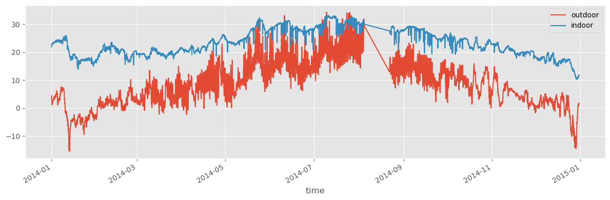
# select january datadf1.info()<class 'pandas.core.frame.DataFrame'>
DatetimeIndex: 49548 entries, 2014-01-01 00:03:06+01:00 to 2014-12-30 23:56:35+01:00
Data columns (total 1 columns):
# Column Non-Null Count Dtype
--- ------ -------------- -----
0 outdoor 49548 non-null float64
dtypes: float64(1)
memory usage: 774.2 KB
df1_jan = df1[(df1.index > "2014-1-1") & (df1.index < "2014-2-1")]df1.index < "2014-2-1"array([ True, True, True, ..., False, False, False], shape=(49548,))df1_jan.info()<class 'pandas.core.frame.DataFrame'>
DatetimeIndex: 4452 entries, 2014-01-01 00:03:06+01:00 to 2014-01-31 23:56:58+01:00
Data columns (total 1 columns):
# Column Non-Null Count Dtype
--- ------ -------------- -----
0 outdoor 4452 non-null float64
dtypes: float64(1)
memory usage: 69.6 KB
df2_jan = df2["2014-1-1":"2014-1-31"]fig, ax = plt.subplots(1, 1, figsize=(12, 4))
df1_jan.plot(ax=ax)
df2_jan.plot(ax=ax)
fig.tight_layout()
fig.savefig("ch12-timeseries-selected-month.pdf")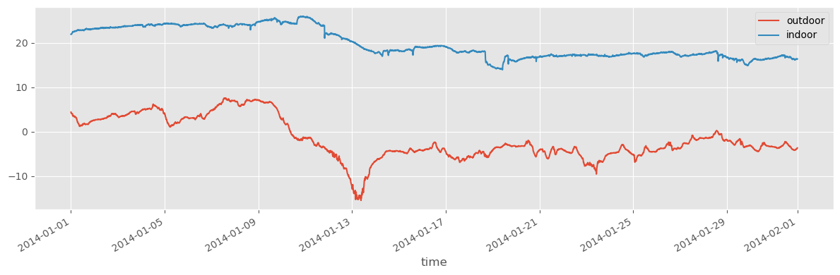
# group by monthdf1_month = df1.reset_index()df1_month["month"] = df1_month.time.apply(lambda x: x.month)df1_month.head()Loading...
df1_month = df1_month[["month", "outdoor"]].groupby("month").aggregate(np.mean)/tmp/ipykernel_73526/982032997.py:1: FutureWarning: The provided callable <function mean at 0x7e4ac0dfbb60> is currently using DataFrameGroupBy.mean. In a future version of pandas, the provided callable will be used directly. To keep current behavior pass the string "mean" instead.
df1_month = df1_month[["month", "outdoor"]].groupby("month").aggregate(np.mean)
df2_month = df2.reset_index()df2_month["month"] = df2_month.time.apply(lambda x: x.month)df2_month = df2_month[["month", "indoor"]].groupby("month").aggregate(np.mean)/tmp/ipykernel_73526/1967358800.py:1: FutureWarning: The provided callable <function mean at 0x7e4ac0dfbb60> is currently using DataFrameGroupBy.mean. In a future version of pandas, the provided callable will be used directly. To keep current behavior pass the string "mean" instead.
df2_month = df2_month[["month", "indoor"]].groupby("month").aggregate(np.mean)
df1_month.head(4)Loading...
df2_month.head(4)Loading...
df_month = df1_month[["outdoor"]].join(df2_month[["indoor"]])df_month.head(3)Loading...
df_month = pd.concat(
[df.to_period("M").groupby(level=0).mean() for df in [df1, df2]], axis=1
)/tmp/ipykernel_73526/1660247247.py:2: UserWarning: Converting to PeriodArray/Index representation will drop timezone information.
[df.to_period("M").groupby(level=0).mean() for df in [df1, df2]], axis=1
df_month.head(3)Loading...
fig, axes = plt.subplots(1, 2, figsize=(12, 4))
df_month.plot(kind="bar", ax=axes[0])
df_month.plot(kind="box", ax=axes[1])
fig.tight_layout()
fig.savefig("ch12-grouped-by-month.pdf")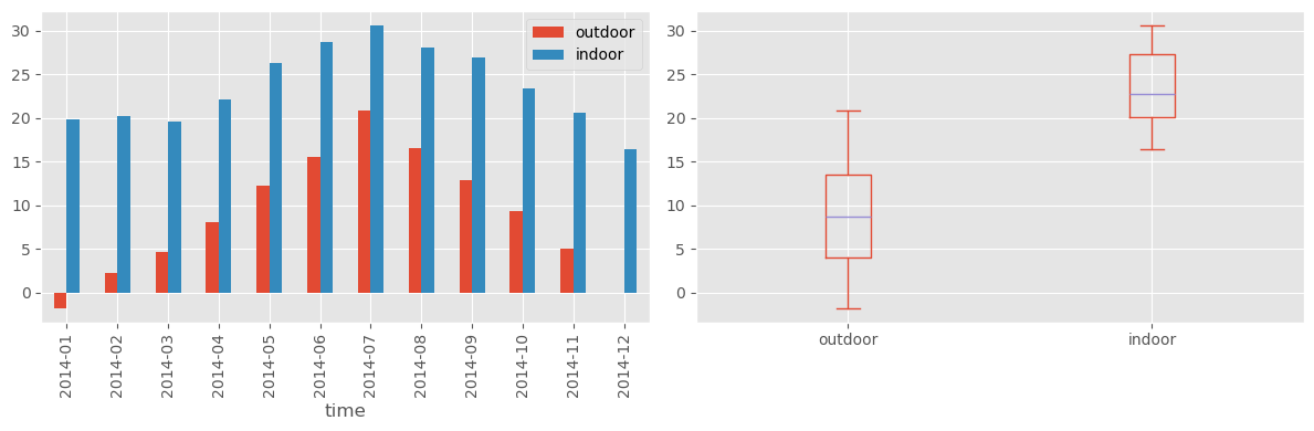
df_monthLoading...
# resamplingdf1_hour = df1.resample("H").mean()/tmp/ipykernel_73526/105550632.py:1: FutureWarning: 'H' is deprecated and will be removed in a future version, please use 'h' instead.
df1_hour = df1.resample("H").mean()
df1_hour.columns = ["outdoor (hourly avg.)"]df1_day = df1.resample("D").mean()df1_day.columns = ["outdoor (daily avg.)"]df1_week = df1.resample("7D").mean()df1_week.columns = ["outdoor (weekly avg.)"]df1_month = df1.resample("M").mean()/tmp/ipykernel_73526/4133909475.py:1: FutureWarning: 'M' is deprecated and will be removed in a future version, please use 'ME' instead.
df1_month = df1.resample("M").mean()
df1_month.columns = ["outdoor (monthly avg.)"]df_diff = df1.resample("D").mean().outdoor - df2.resample("D").mean().indoorfig, (ax1, ax2) = plt.subplots(2, 1, figsize=(12, 6))
df1_hour.plot(ax=ax1, alpha=0.25)
df1_day.plot(ax=ax1)
df1_week.plot(ax=ax1)
df1_month.plot(ax=ax1)
df_diff.plot(ax=ax2)
ax2.set_title("temperature difference between outdoor and indoor")
fig.tight_layout()
fig.savefig("ch12-timeseries-resampled.pdf")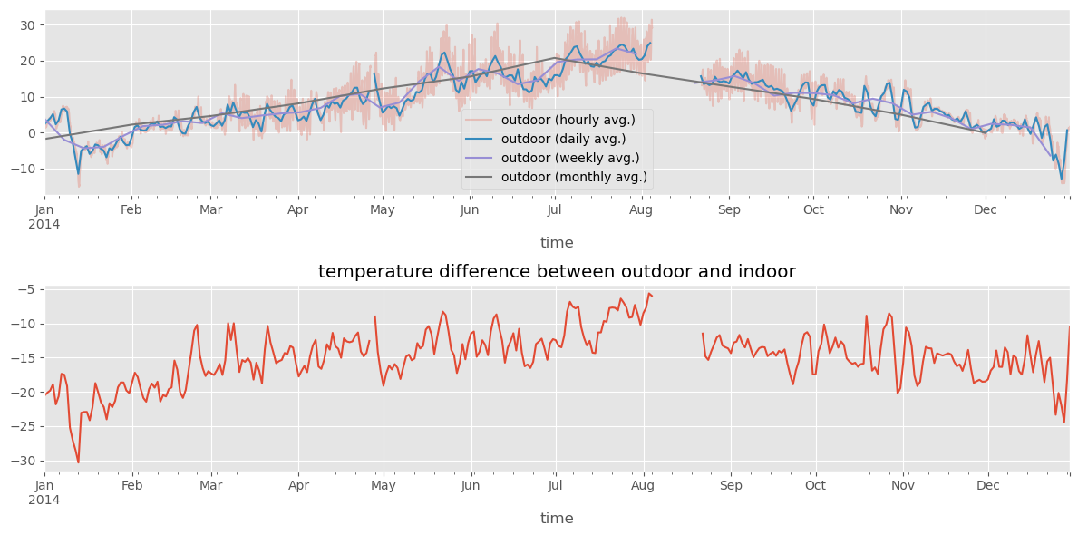
pd.concat(
[
df1.resample("5min").mean().rename(columns={"outdoor": "None"}),
df1.resample("5min").ffill().rename(columns={"outdoor": "ffill"}),
df1.resample("5min").bfill().rename(columns={"outdoor": "bfill"}),
],
axis=1,
).head()Loading...
Selected day
df1_dec25 = df1[(df1.index < "2014-9-1") & (df1.index >= "2014-8-1")].resample("D")df1_dec25 = df1.loc["2014-12-25"]df1_dec25.head(5)Loading...
df2_dec25 = df2.loc["2014-12-25"]df2_dec25.head(5)Loading...
df1_dec25.describe().TLoading...
fig, ax = plt.subplots(1, 1, figsize=(12, 4))
df1_dec25.plot(ax=ax)
fig.savefig("ch12-timeseries-selected-month-12.pdf")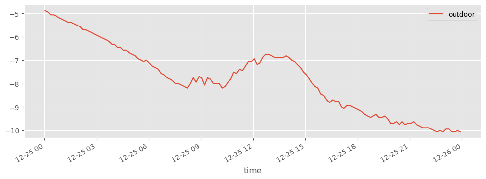
df1.indexDatetimeIndex(['2014-01-01 00:03:06+01:00', '2014-01-01 00:13:06+01:00',
'2014-01-01 00:23:07+01:00', '2014-01-01 00:33:07+01:00',
'2014-01-01 00:43:08+01:00', '2014-01-01 00:53:08+01:00',
'2014-01-01 01:03:09+01:00', '2014-01-01 01:13:09+01:00',
'2014-01-01 01:23:10+01:00', '2014-01-01 01:33:26+01:00',
...
'2014-12-30 22:26:30+01:00', '2014-12-30 22:36:31+01:00',
'2014-12-30 22:46:31+01:00', '2014-12-30 22:56:32+01:00',
'2014-12-30 23:06:32+01:00', '2014-12-30 23:16:33+01:00',
'2014-12-30 23:26:33+01:00', '2014-12-30 23:36:34+01:00',
'2014-12-30 23:46:35+01:00', '2014-12-30 23:56:35+01:00'],
dtype='datetime64[ns, Europe/Stockholm]', name='time', length=49548, freq=None)Seaborn statistical visualization library
sns.set(style="darkgrid")# sns.set(style="whitegrid")df1 = pd.read_csv(
"temperature_outdoor_2014.tsv", delimiter="\t", names=["time", "outdoor"]
)
df1.time = (
pd.to_datetime(df1.time.values, unit="s")
.tz_localize("UTC")
.tz_convert("Europe/Stockholm")
)
df1 = df1.set_index("time").resample("10min").mean()
df2 = pd.read_csv(
    "temperature_indoor_2014.tsv", delimiter="\t", names=["time", "indoor"]
)
df2.time = (
    pd.to_datetime(df2.time.values, unit="s")
    .tz_localize("UTC")
    .tz_convert("Europe/Stockholm")
)
df2 = df2.set_index("time").resample("10min").mean()
df_temp = pd.concat([df1, df2], axis=1)fig, ax = plt.subplots(1, 1, figsize=(8, 4))
df_temp.resample("D").mean().plot(y=["outdoor", "indoor"], ax=ax)
fig.tight_layout()
fig.savefig("ch12-seaborn-plot.pdf")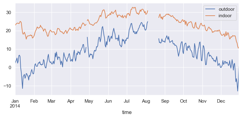
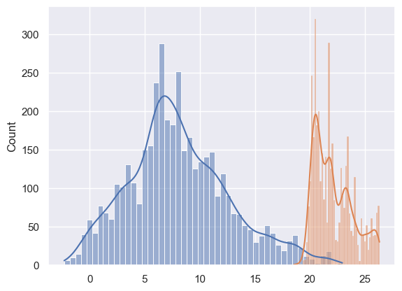
# sns.kdeplot(df_temp["outdoor"].dropna().values, shade=True, cumulative=True);sns.histplot(
df_temp.to_period("M")["outdoor"]["2014-04"].dropna().values, bins=50, kde=True
)
sns.histplot(
df_temp.to_period("M")["indoor"]["2014-04"].dropna().values, bins=50, kde=True
)
plt.savefig("ch12-seaborn-distplot.pdf")/tmp/ipykernel_73526/257196248.py:2: UserWarning: Converting to PeriodArray/Index representation will drop timezone information.
df_temp.to_period("M")["outdoor"]["2014-04"].dropna().values, bins=50, kde=True
/tmp/ipykernel_73526/257196248.py:5: UserWarning: Converting to PeriodArray/Index representation will drop timezone information.
df_temp.to_period("M")["indoor"]["2014-04"].dropna().values, bins=50, kde=True
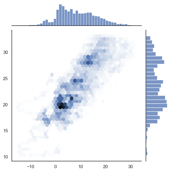
with sns.axes_style("white"):
    sns.jointplot(
        x=df_temp.resample("H").mean()["outdoor"].values,
        y=df_temp.resample("H").mean()["indoor"].values,
        kind="hex",
    )

plt.savefig("ch12-seaborn-jointplot.pdf")
/tmp/ipykernel_73526/3899608506.py:3: FutureWarning: 'H' is deprecated and will be removed in a future version, please use 'h' instead.
x=df_temp.resample("H").mean()["outdoor"].values,
/tmp/ipykernel_73526/3899608506.py:4: FutureWarning: 'H' is deprecated and will be removed in a future version, please use 'h' instead.
y=df_temp.resample("H").mean()["indoor"].values,
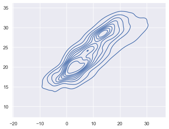
sns.kdeplot(
    x=df_temp.resample("H").mean()["outdoor"].dropna().values,
    y=df_temp.resample("H").mean()["indoor"].dropna().values,
    fill=False,
)
plt.savefig("ch12-seaborn-kdeplot.pdf")
/tmp/ipykernel_73526/3128183993.py:2: FutureWarning: 'H' is deprecated and will be removed in a future version, please use 'h' instead.
x=df_temp.resample("H").mean()["outdoor"].dropna().values,
/tmp/ipykernel_73526/3128183993.py:3: FutureWarning: 'H' is deprecated and will be removed in a future version, please use 'h' instead.
y=df_temp.resample("H").mean()["indoor"].dropna().values,
fig, (ax1, ax2) = plt.subplots(1, 2, figsize=(8, 4))

sns.boxplot(df_temp.dropna(), ax=ax1, palette="pastel")
sns.violinplot(df_temp.dropna(), ax=ax2, palette="pastel")

fig.tight_layout()
fig.savefig("ch12-seaborn-boxplot-violinplot.pdf")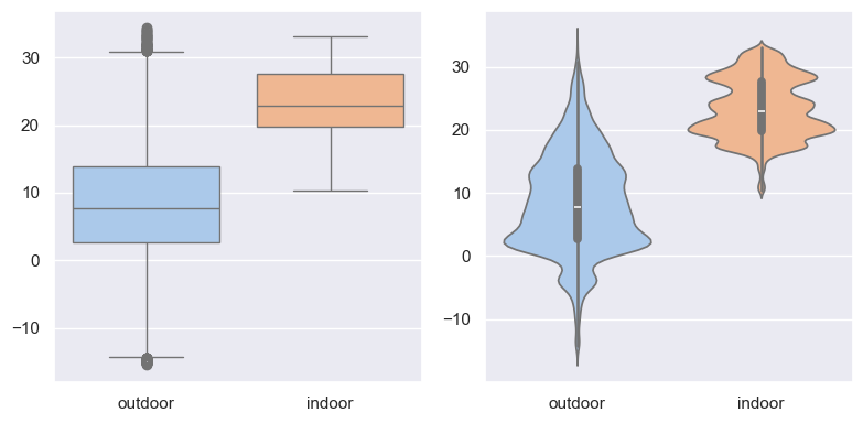
sns.violinplot(
    x=df_temp.dropna().index.month, y=df_temp.dropna().outdoor, color="skyblue"
)
plt.savefig("ch12-seaborn-violinplot.pdf")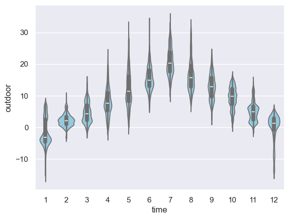
df_temp["month"] = df_temp.index.month
df_temp["hour"] = df_temp.index.hourdf_temp.head()Loading...
table = pd.pivot_table(
    df_temp, values="outdoor", index=["month"], columns=["hour"], aggfunc=np.mean
)
/tmp/ipykernel_73526/2254952302.py:1: FutureWarning: The provided callable <function mean at 0x7e4ac0dfbb60> is currently using DataFrameGroupBy.mean. In a future version of pandas, the provided callable will be used directly. To keep current behavior pass the string "mean" instead.
table = pd.pivot_table(
tableLoading...
fig, ax = plt.subplots(1, 1, figsize=(8, 4))
sns.heatmap(table, ax=ax)
fig.tight_layout()
fig.savefig("ch12-seaborn-heatmap.pdf")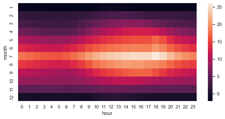
- Johansson, R. (2024). Numerical Python: Scientific Computing and Data Science Applications with Numpy, SciPy and Matplotlib. Apress. 10.1007/979-8-8688-0413-7