Chapter 8: Integration

Robert Johansson

Source code listings for Numerical Python - Scientific Computing and Data Science Applications with Numpy, SciPy and Matplotlib (ISBN 979-8-8688-0412-0).

%matplotlib inline
import matplotlib as mpl
import matplotlib.pyplot as plt

mpl.rcParams["mathtext.fontset"] = "stix"
mpl.rcParams["font.family"] = "serif"
mpl.rcParams["font.sans-serif"] = "stix"

import numpy as np

from scipy import integrate

import mpmath
import sympy

sympy.init_printing()

Simpson’s rule¶

a, b, X = sympy.symbols("a, b, x")
f = sympy.Function("f")

# x = a, (a+b)/3, 2 * (a+b)/3, b # 3rd order quadrature rule
x = a, (a + b) / 2, b  # simpson's rule
# x = a, b # trapezoid rule
# x = ((b+a)/2,)  # mid-point rule

w = [sympy.symbols("w_%d" % i) for i in range(len(x))]

q_rule = sum([w[i] * f(x[i]) for i in range(len(x))])

q_rule

phi = [sympy.Lambda(X, X**n) for n in range(len(x))]

phi

eqs = [
    q_rule.subs(f, phi[n]) - sympy.integrate(phi[n](X), (X, a, b))
    for n in range(len(phi))
]

eqs

w_sol = sympy.solve(eqs, w)

w_sol

q_rule.subs(w_sol).simplify()

SciPy `integrate`¶

Simple integration example¶

def f(x):
    return np.exp(-(x**2))

val, err = integrate.quad(f, -1, 1)

val

err

Extra arguments¶

def f(x, a, b, c):
    return a * np.exp(-(((x - b) / c) ** 2))

val, err = integrate.quad(f, -1, 1, args=(1, 2, 3))

val

err

Reshuffle arguments¶

from scipy.special import jv

val, err = integrate.quad(lambda x: jv(0, x), 0, 5)

val

err

Infinite limits¶

f = lambda x: np.exp(-(x**2))

val, err = integrate.quad(f, -np.inf, np.inf)

val

err

Singularity¶

f = lambda x: 1 / np.sqrt(abs(x))

a, b = -1, 1

integrate.quad(f, a, b)

/tmp/ipykernel_40722/592522017.py:1: RuntimeWarning: divide by zero encountered in scalar divide
  f = lambda x: 1 / np.sqrt(abs(x))

integrate.quad(f, a, b, points=[0])

fig, ax = plt.subplots(figsize=(8, 3))

x = np.linspace(a, b, 10000)
ax.plot(x, f(x), lw=2)
ax.fill_between(x, f(x), color="green", alpha=0.5)
ax.set_xlabel("$x$", fontsize=18)
ax.set_ylabel("$f(x)$", fontsize=18)
ax.set_ylim(0, 25)
ax.set_xlim(-1, 1)

fig.tight_layout()
fig.savefig("ch8-diverging-integrand.pdf")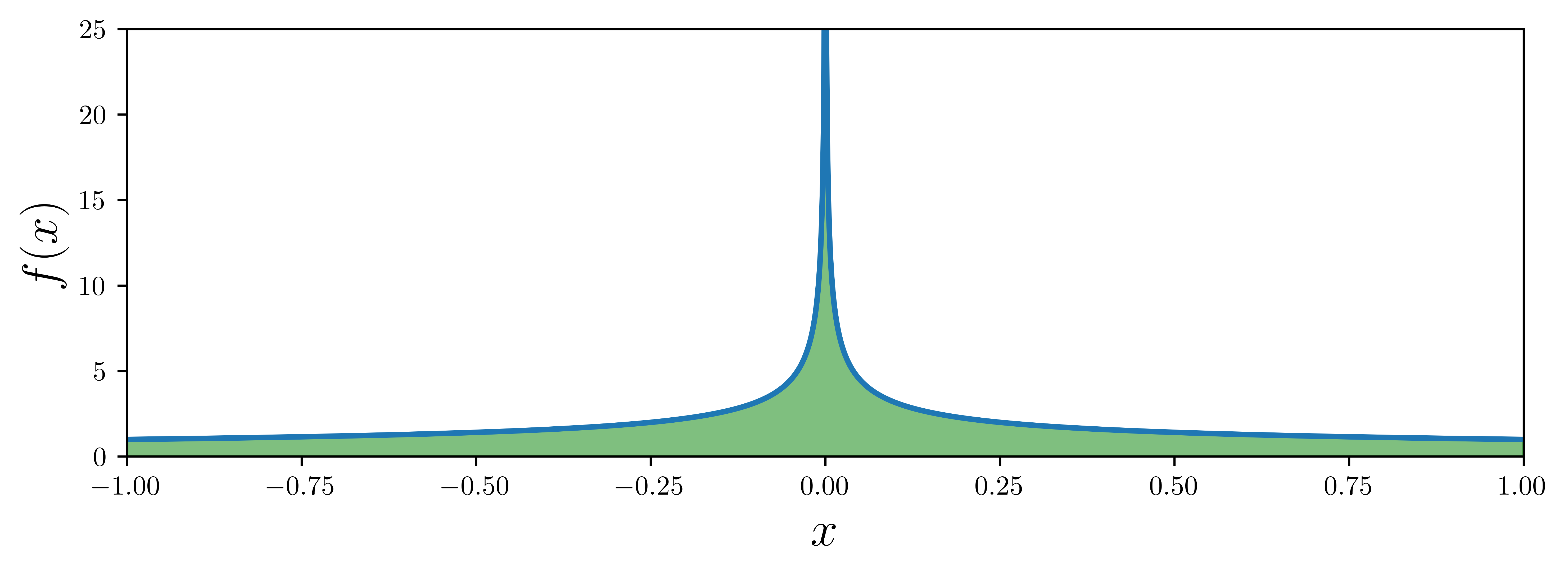

Tabulated integrand¶

f = lambda x: np.sqrt(x)

a, b = 0, 2

x = np.linspace(a, b, 25)

y = f(x)

fig, ax = plt.subplots(figsize=(8, 3))
ax.plot(x, y, "bo")
xx = np.linspace(a, b, 500)
ax.plot(xx, f(xx), "b-")
ax.fill_between(xx, f(xx), color="green", alpha=0.5)
ax.set_xlabel(r"$x$", fontsize=18)
ax.set_ylabel(r"$f(x)$", fontsize=18)
fig.tight_layout()
fig.savefig("ch8-tabulated-integrand.pdf")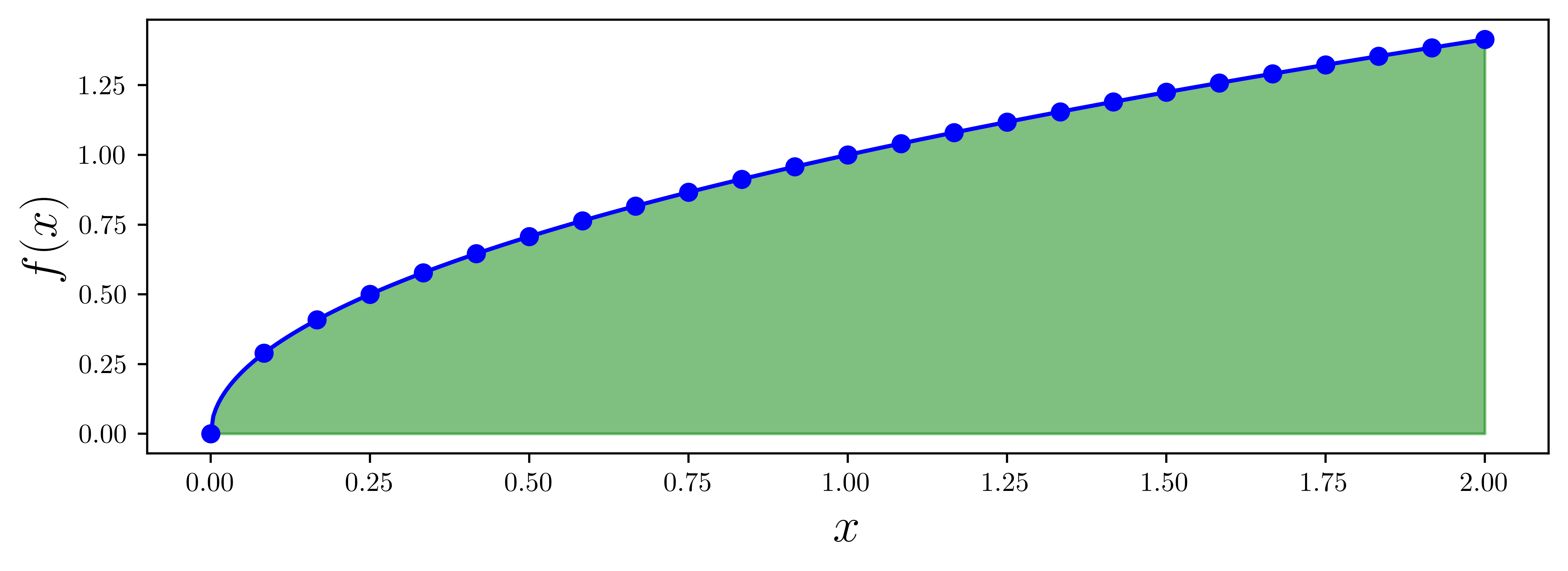

val_trapz = integrate.trapezoid(y, x)

val_trapz

val_simps = integrate.simpson(y, x)

val_simps

val_exact = 2.0 / 3.0 * (b - a) ** (3.0 / 2.0)

val_exact

val_exact - val_trapz

val_exact - val_simps

x = np.linspace(a, b, 1 + 2**6)

len(x)

y = f(x)

val_exact - integrate.romb(y, dx=(x[1] - x[0]))

val_exact - integrate.simpson(y, dx=x[1] - x[0])

Higher dimension¶

def f(x):
    return np.exp(-(x**2))

%time integrate.quad(f, a, b)

CPU times: user 49 μs, sys: 4 μs, total: 53 μs
Wall time: 57.7 μs

def f(x, y):
    return np.exp(-(x**2) - y**2)

a, b = 0, 1

g = lambda x: 0

h = lambda x: 1

integrate.dblquad(f, a, b, g, h)

integrate.dblquad(lambda x, y: np.exp(-(x**2) - y**2), 0, 1, lambda x: 0, lambda x: 1)

fig, ax = plt.subplots(figsize=(6, 5))

x = y = np.linspace(-1.25, 1.25, 75)
X, Y = np.meshgrid(x, y)

c = ax.contour(X, Y, f(X, Y), 15, cmap=mpl.cm.RdBu, vmin=-1, vmax=1)

bound_rect = plt.Rectangle((0, 0), 1, 1, facecolor="grey")
ax.add_patch(bound_rect)

ax.axis("tight")
ax.set_xlabel("$x$", fontsize=18)
ax.set_ylabel("$y$", fontsize=18)

fig.tight_layout()
fig.savefig("ch8-multi-dim-integrand.pdf")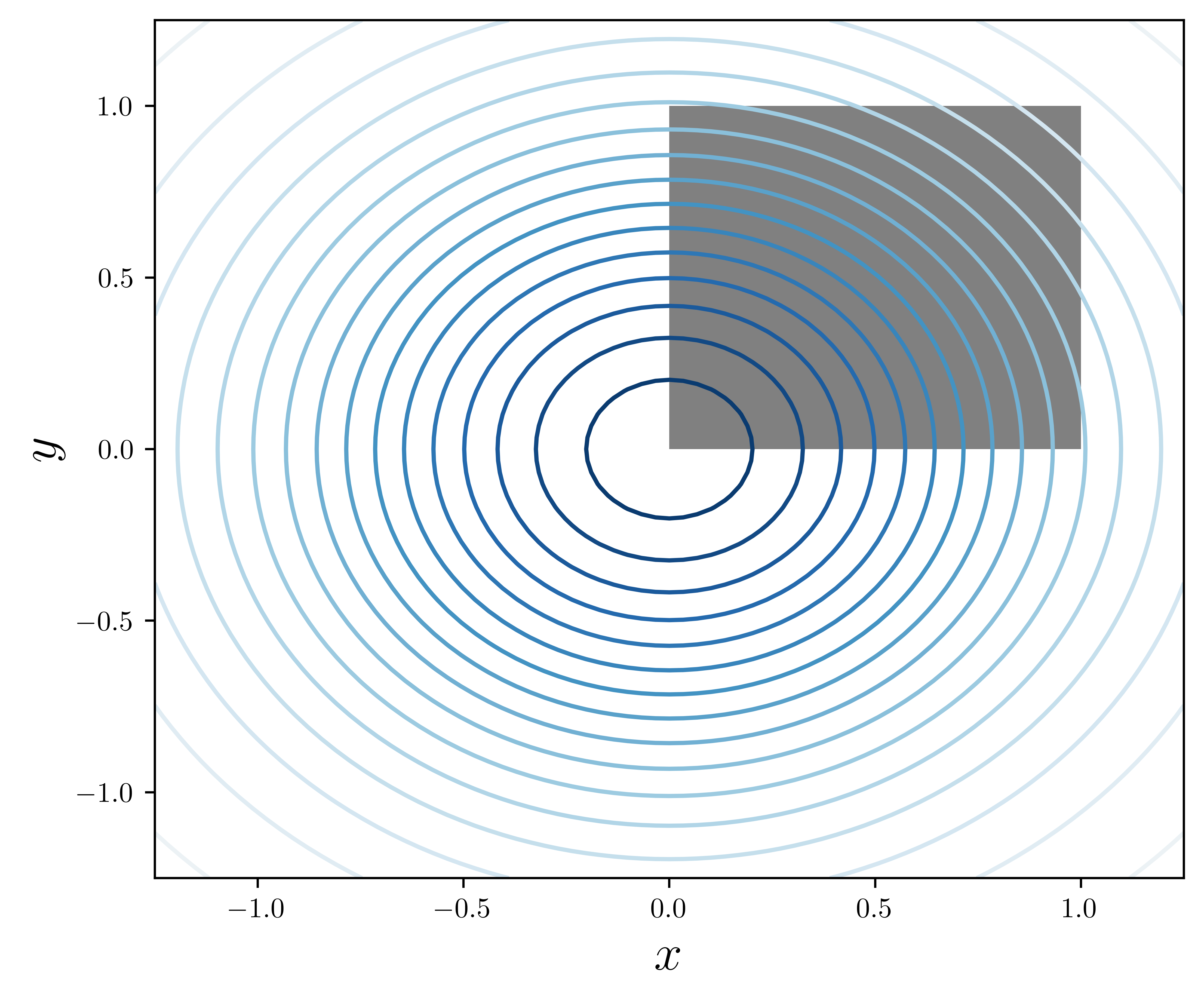

integrate.dblquad(f, 0, 1, lambda x: -1 + x, lambda x: 1 - x)

def f(x, y, z):
    return np.exp(-(x**2) - y**2 - z**2)

integrate.tplquad(f, 0, 1, lambda x: 0, lambda x: 1, lambda x, y: 0, lambda x, y: 1)

integrate.nquad(f, [(0, 1), (0, 1), (0, 1)])

nquad¶

def f(*args):
    return np.exp(-np.sum(np.array(args) ** 2))

%time integrate.nquad(f, [(0,1)] * 1)

CPU times: user 322 μs, sys: 23 μs, total: 345 μs
Wall time: 350 μs

%time integrate.nquad(f, [(0,1)] * 2)

CPU times: user 1.86 ms, sys: 136 μs, total: 1.99 ms
Wall time: 1.99 ms

%time integrate.nquad(f, [(0,1)] * 3)

CPU times: user 55.4 ms, sys: 0 ns, total: 55.4 ms
Wall time: 55.2 ms

%time integrate.nquad(f, [(0,1)] * 4)

CPU times: user 696 ms, sys: 149 μs, total: 696 ms
Wall time: 697 ms

%time integrate.nquad(f, [(0,1)] * 5)

CPU times: user 15.3 s, sys: 5.31 ms, total: 15.3 s
Wall time: 15.3 s

Monte Carlo integration¶

from skmonaco import mcquad

%time val, err = mcquad(f, xl=np.zeros(5), xu=np.ones(5), npoints=100000)

CPU times: user 440 ms, sys: 3.26 ms, total: 444 ms
Wall time: 447 ms

val, err

%time val, err = mcquad(f, xl=np.zeros(10), xu=np.ones(10), npoints=100000)

CPU times: user 466 ms, sys: 0 ns, total: 466 ms
Wall time: 469 ms

val, err

Symbolic and multi-precision quadrature¶

x = sympy.symbols("x")

f = 2 * sympy.sqrt(1 - x**2)

a, b = -1, 1

sympy.plot(f, (x, -2, 2));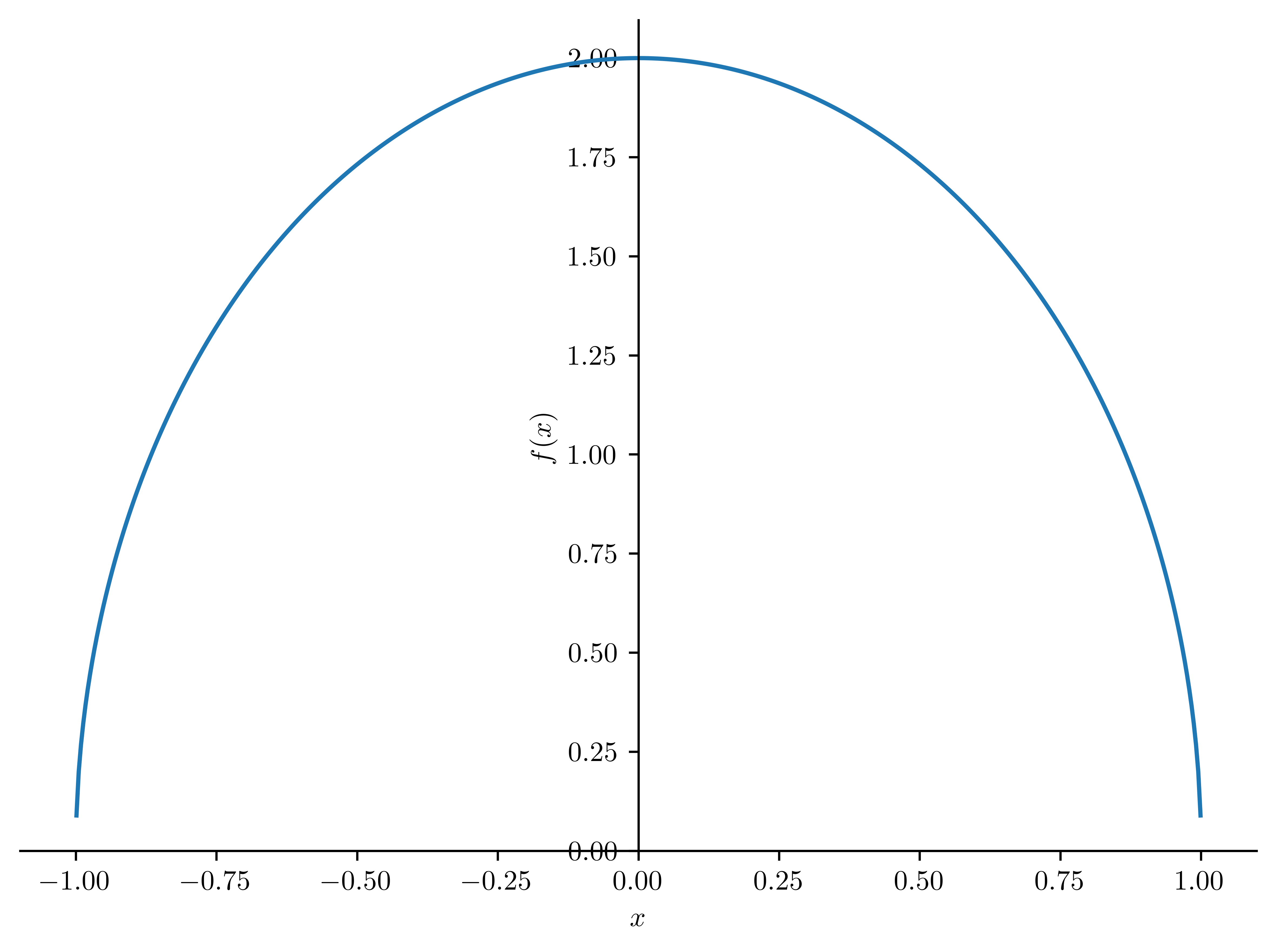

val_sym = sympy.integrate(f, (x, a, b))

val_sym

mpmath.mp.dps = 75

f_mpmath = sympy.lambdify(x, f, "mpmath")

val = mpmath.quad(f_mpmath, (a, b))

sympy.sympify(val)

sympy.N(val_sym, mpmath.mp.dps + 1) - val

%timeit mpmath.quad(f_mpmath, [a, b])

1.64 ms ± 11.7 μs per loop (mean ± std. dev. of 7 runs, 1,000 loops each)

f_numpy = sympy.lambdify(x, f, "numpy")

%timeit integrate.quad(f_numpy, a, b)

134 μs ± 2.25 μs per loop (mean ± std. dev. of 7 runs, 10,000 loops each)

double and triple integrals¶

def f2(x, y):
    return np.cos(x) * np.cos(y) * np.exp(-(x**2) - y**2)


def f3(x, y, z):
    return np.cos(x) * np.cos(y) * np.cos(z) * np.exp(-(x**2) - y**2 - z**2)

integrate.dblquad(f2, 0, 1, lambda x: 0, lambda x: 1)

integrate.tplquad(f3, 0, 1, lambda x: 0, lambda x: 1, lambda x, y: 0, lambda x, y: 1)

x, y, z = sympy.symbols("x, y, z")

f2 = sympy.cos(x) * sympy.cos(y) * sympy.exp(-(x**2) - y**2)

f3 = sympy.cos(x) * sympy.cos(y) * sympy.cos(z) * sympy.exp(-(x**2) - y**2 - z**2)

sympy.integrate(f3, (x, 0, 1), (y, 0, 1), (z, 0, 1))  # this does not succeed

f2_numpy = sympy.lambdify((x, y), f2, "numpy")

integrate.dblquad(f2_numpy, 0, 1, lambda x: 0, lambda x: 1)

f3_numpy = sympy.lambdify((x, y, z), f3, "numpy")

integrate.tplquad(
    f3_numpy, 0, 1, lambda x: 0, lambda x: 1, lambda x, y: 0, lambda x, y: 1
)

mpmath.mp.dps = 30

f2_mpmath = sympy.lambdify((x, y), f2, "mpmath")

res = mpmath.quad(f2_mpmath, (0, 1), (0, 1))
res

mpf('0.430564794306099099242308990195783')

f3_mpmath = sympy.lambdify((x, y, z), f3, "mpmath")

res = mpmath.quad(f3_mpmath, (0, 1), (0, 1), (0, 1))

sympy.sympify(res)

%time res = sympy.sympify(mpmath.quad(f3_mpmath, (0, 1), (0, 1), (0, 1)))

CPU times: user 47.1 s, sys: 3.37 ms, total: 47.1 s
Wall time: 47.2 s

Line integrals¶

t, x, y = sympy.symbols("t, x, y")

C = sympy.Curve([sympy.cos(t), sympy.sin(t)], (t, 0, 2 * sympy.pi))

sympy.line_integrate(1, C, [x, y])

sympy.line_integrate(x**2 * y**2, C, [x, y])

Integral transformations¶

Laplace transforms¶

s = sympy.symbols("s")

a, t = sympy.symbols("a, t", positive=True)

f = sympy.sin(a * t)

sympy.laplace_transform(f, t, s)

F = sympy.laplace_transform(f, t, s, noconds=True)

sympy.inverse_laplace_transform(F, s, t, noconds=True)

[sympy.laplace_transform(f, t, s, noconds=True) for f in [t, t**2, t**3, t**4]]

n = sympy.symbols("n", integer=True, positive=True)

sympy.laplace_transform(t**n, t, s, noconds=True)

sympy.laplace_transform((1 - a * t) * sympy.exp(-a * t), t, s, noconds=True)

Fourier Transforms¶

w = sympy.symbols("omega")

f = sympy.exp(-a * t**2)

F = sympy.fourier_transform(f, t, w)

sympy.inverse_fourier_transform(F, w, t)

sympy.fourier_transform(sympy.cos(t), t, w)  # not good

References¶

Johansson, R. (2024). Numerical Python: Scientific Computing and Data Science Applications with Numpy, SciPy and Matplotlib. Apress. 10.1007/979-8-8688-0413-7

Simpson’s rule¶

SciPy integrate¶

Simple integration example¶

Extra arguments¶

Reshuffle arguments¶

Infinite limits¶

Singularity¶

Tabulated integrand¶

Higher dimension¶

nquad¶

Monte Carlo integration¶

Symbolic and multi-precision quadrature¶

double and triple integrals¶

Line integrals¶

Integral transformations¶

Laplace transforms¶

Fourier Transforms¶

SciPy `integrate`¶