%matplotlib inline

# %config InlineBackend.figure_format='retina'
# %config InlineBackend.figure_format='svg'

import matplotlib as mpl
import matplotlib.pyplot as plt
# mpl.rcParams['mathtext.fontset'] = 'stix'
# mpl.rcParams['font.family'] = 'serif'
# mpl.rcParams['font.sans-serif'] = 'stix'

import numpy as np

x = np.linspace(-5, 2, 100)

y1 = x**3 + 5 * x**2 + 10

y2 = 3 * x**2 + 10 * x

y3 = 6 * x + 10

fig, ax = plt.subplots()

ax.plot(x, y1, color="blue", label="y(x)")
ax.plot(x, y2, color="red", label="y'(x)")
ax.plot(x, y3, color="green", label="y''(x)")

ax.set_xlabel("x")
ax.set_ylabel("y")
ax.legend()

fig.savefig("ch4-figure-1.pdf")

mpl.rcParams["font.family"] = "serif"
mpl.rcParams["font.size"] = "12"

fig, ax = plt.subplots()

ax.plot(x, y1, lw=1.5, color="blue", label=r"$y(x)$")
ax.plot(x, y2, lw=1.5, color="red", label=r"$y'(x)$")
ax.plot(x, y3, lw=1.5, color="green", label=r"$y''(x)$")

ax.plot(x, np.zeros_like(x), lw=0.5, color="black")
ax.plot(
    [-3.33, -3.33],
    [0, (-3.3) ** 3 + 5 * (-3.3) ** 2 + 10],
    ls="--",
    lw=0.5,
    color="black",
)
ax.plot([0, 0], [0, 10], lw=0.5, ls="--", color="black")
ax.plot([0], [10], lw=0.5, marker="o", color="blue")
ax.plot([-3.33], [(-3.3) ** 3 + 5 * (-3.3) ** 2 + 10], lw=0.5, marker="o", color="blue")

ax.set_ylim(-15, 40)
ax.set_yticks([-10, 0, 10, 20, 30])
ax.set_xticks([-4, -2, 0, 2])

ax.set_xlabel("$x$", fontsize=18)
ax.set_ylabel("$y$", fontsize=18)
ax.legend(loc=0, ncol=3, fontsize=14, frameon=False)

fig.tight_layout();

fig.savefig("ch4-figure-2.pdf")

mpl.rcParams["font.family"] = "sans-serif"
mpl.rcParams["font.size"] = "10"

%matplotlib inline
# %config InlineBackend.figure_format='svg'
%config InlineBackend.figure_format='retina'

import matplotlib as mpl

# mpl.use('qt4agg')
import matplotlib.pyplot as plt
import numpy as np

x = np.linspace(-5, 2, 100)
y1 = x**3 + 5 * x**2 + 10
y2 = 3 * x**2 + 10 * x
y3 = 6 * x + 10

fig, ax = plt.subplots()

ax.plot(x, y1, color="blue", label="y(x)")
ax.plot(x, y2, color="red", label="y'(x)")
ax.plot(x, y3, color="green", label="y''(x)")

ax.set_xlabel("x")
ax.set_ylabel("y")
ax.legend()

plt.show()

fig = plt.figure(figsize=(8, 2.5), facecolor="#f1f1f1")

# axes coordinates as fractions of the canvas width and height
left, bottom, width, height = 0.1, 0.1, 0.8, 0.8
ax = fig.add_axes((left, bottom, width, height), facecolor="#e1e1e1")

x = np.linspace(-2, 2, 1000)
y1 = np.cos(40 * x)
y2 = np.exp(-(x**2))

ax.plot(x, y1 * y2)
ax.plot(x, y2, "g")
ax.plot(x, -y2, "g")
ax.set_xlabel("x")
ax.set_ylabel("y")

fig.savefig("ch4-graph.png", dpi=100)  # , facecolor="red")
fig.savefig("ch4-graph.pdf", dpi=300, facecolor="#f1f1f1")

fignum = 0


def hide_labels(fig, ax):
    global fignum
    ax.set_xticks([])
    ax.set_yticks([])
    ax.xaxis.set_ticks_position("none")
    ax.yaxis.set_ticks_position("none")
    ax.axis("tight")

    fignum += 1
    fig.savefig("ch4-plot-types-%d.pdf" % fignum)

x = np.linspace(-3, 3, 25)
y1 = x**3 + 3 * x**2 + 10
y2 = -1.5 * x**3 + 10 * x**2 - 15

fig, ax = plt.subplots(figsize=(4, 3))

ax.plot(x, y1)
ax.plot(x, y2)

hide_labels(fig, ax)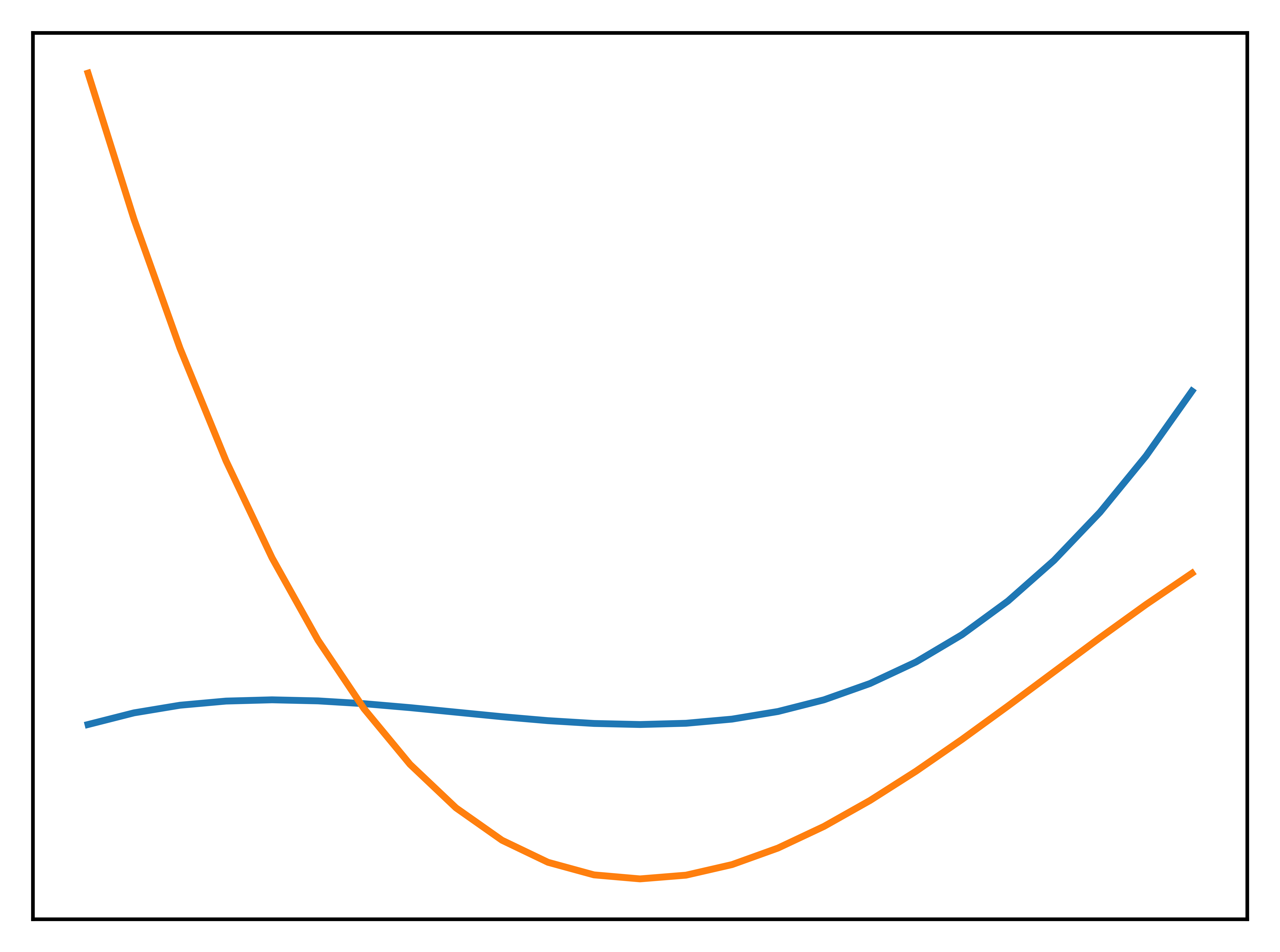

fig, ax = plt.subplots(figsize=(4, 3))

ax.step(x, y1)
ax.step(x, y2)

hide_labels(fig, ax)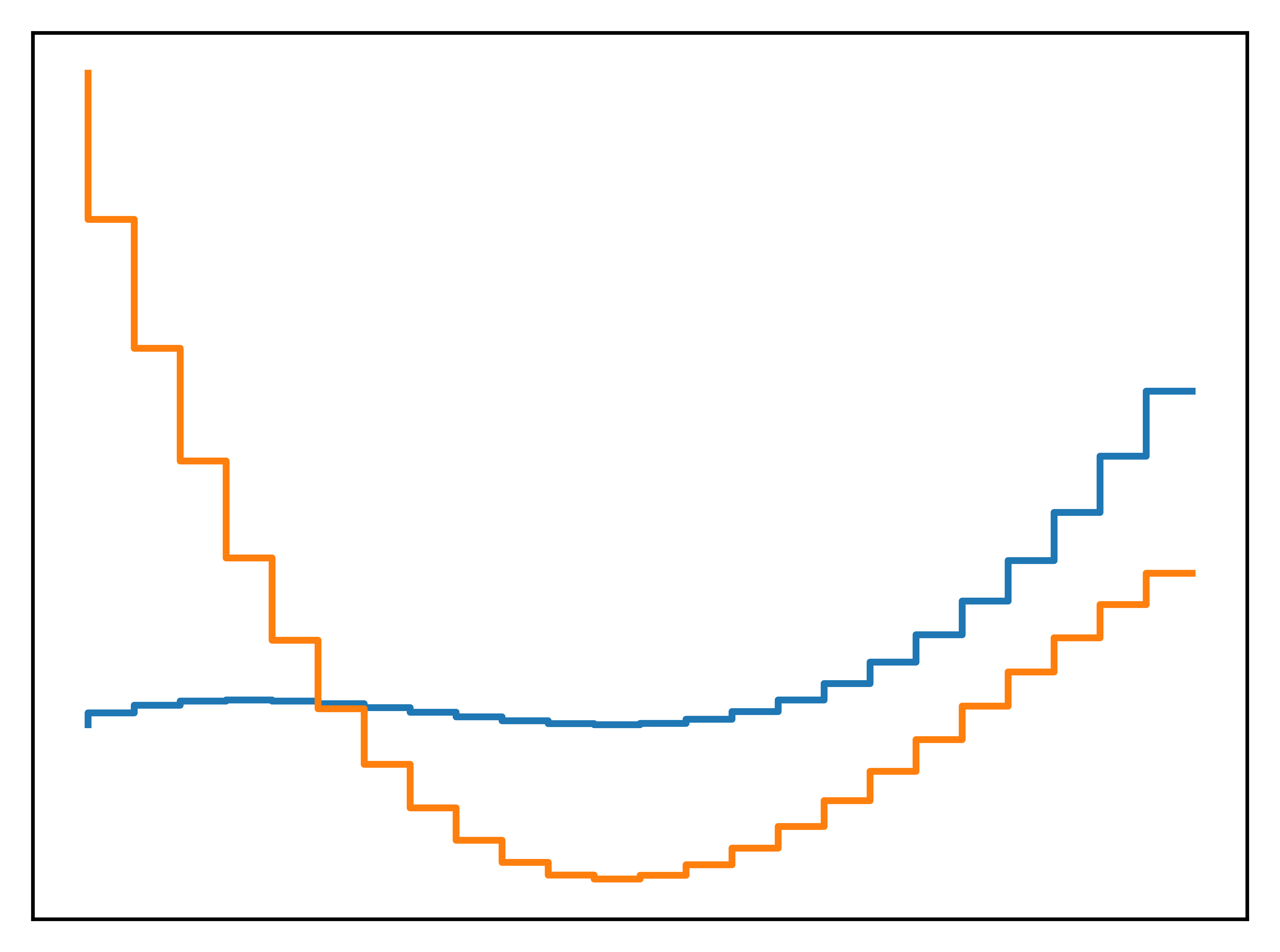

fig, ax = plt.subplots(figsize=(4, 3))
width = 6 / 50.0
ax.bar(x - width / 2, y1, width=width, color="blue")
ax.bar(x + width / 2, y2, width=width, color="green")

hide_labels(fig, ax)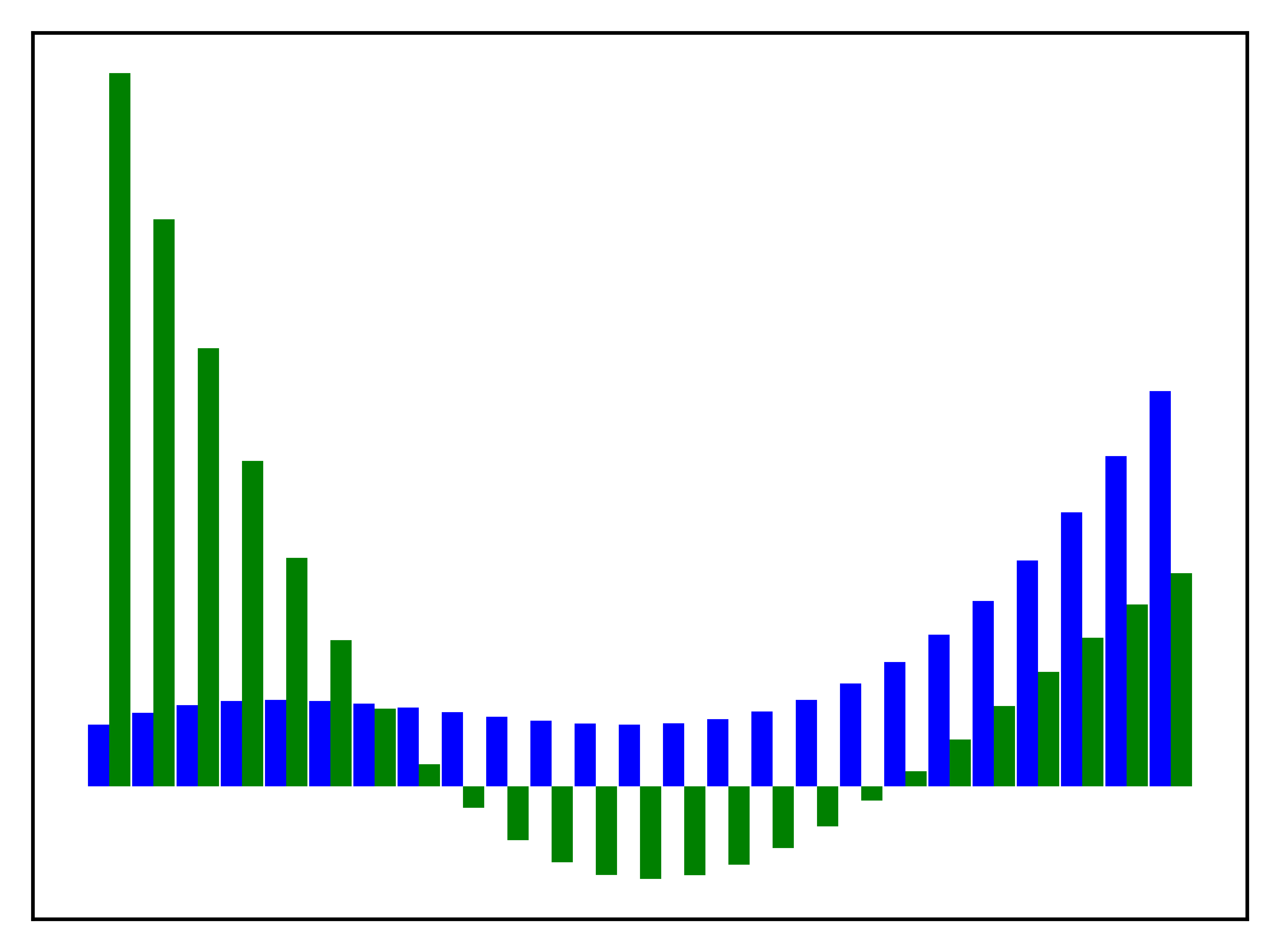

fig, ax = plt.subplots(figsize=(4, 3))
ax.fill_between(x, y1, y2)

hide_labels(fig, ax)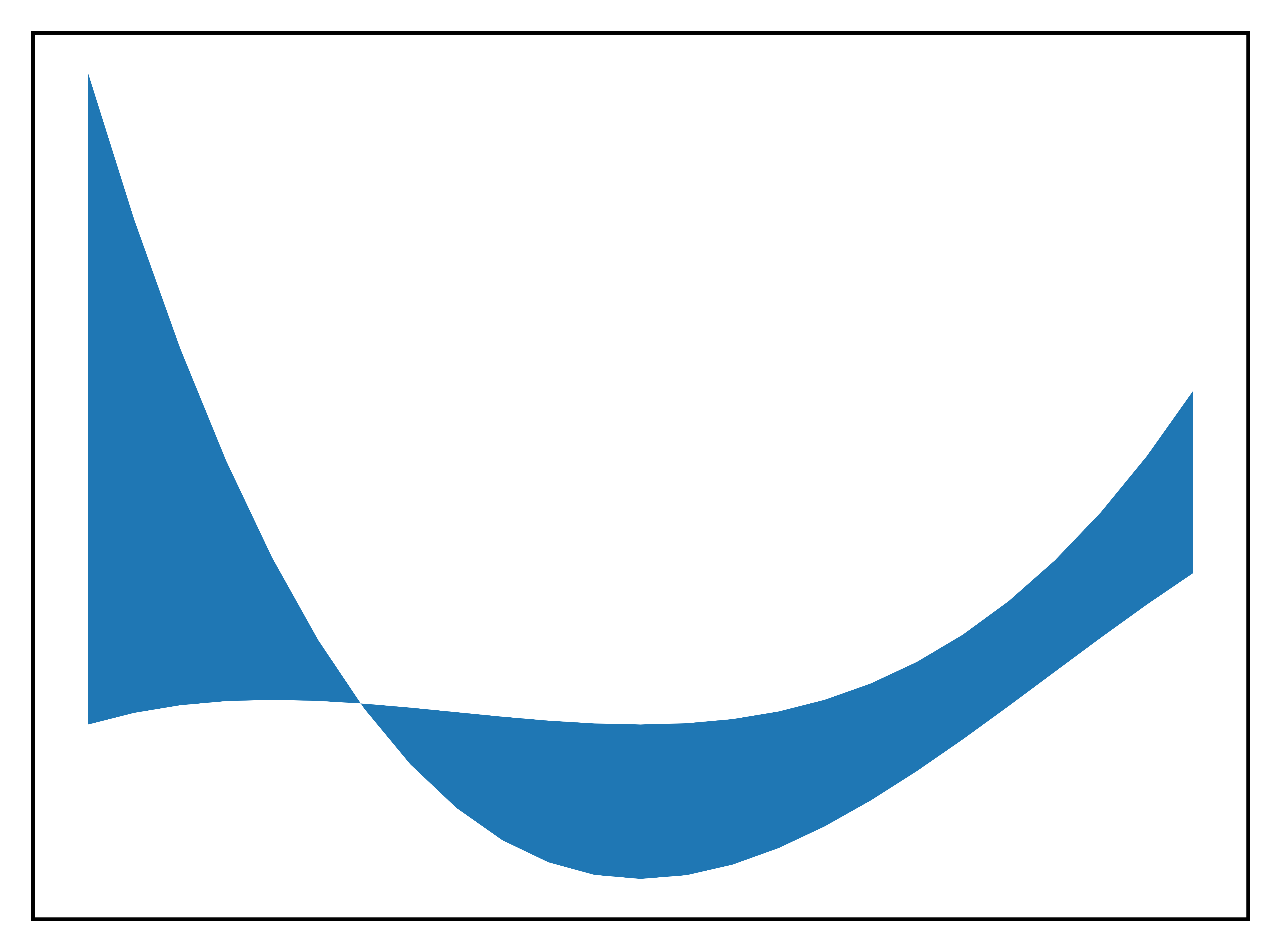

fig, ax = plt.subplots(figsize=(4, 3))
ax.hist(y2, bins=30)
ax.hist(y1, bins=30)

hide_labels(fig, ax)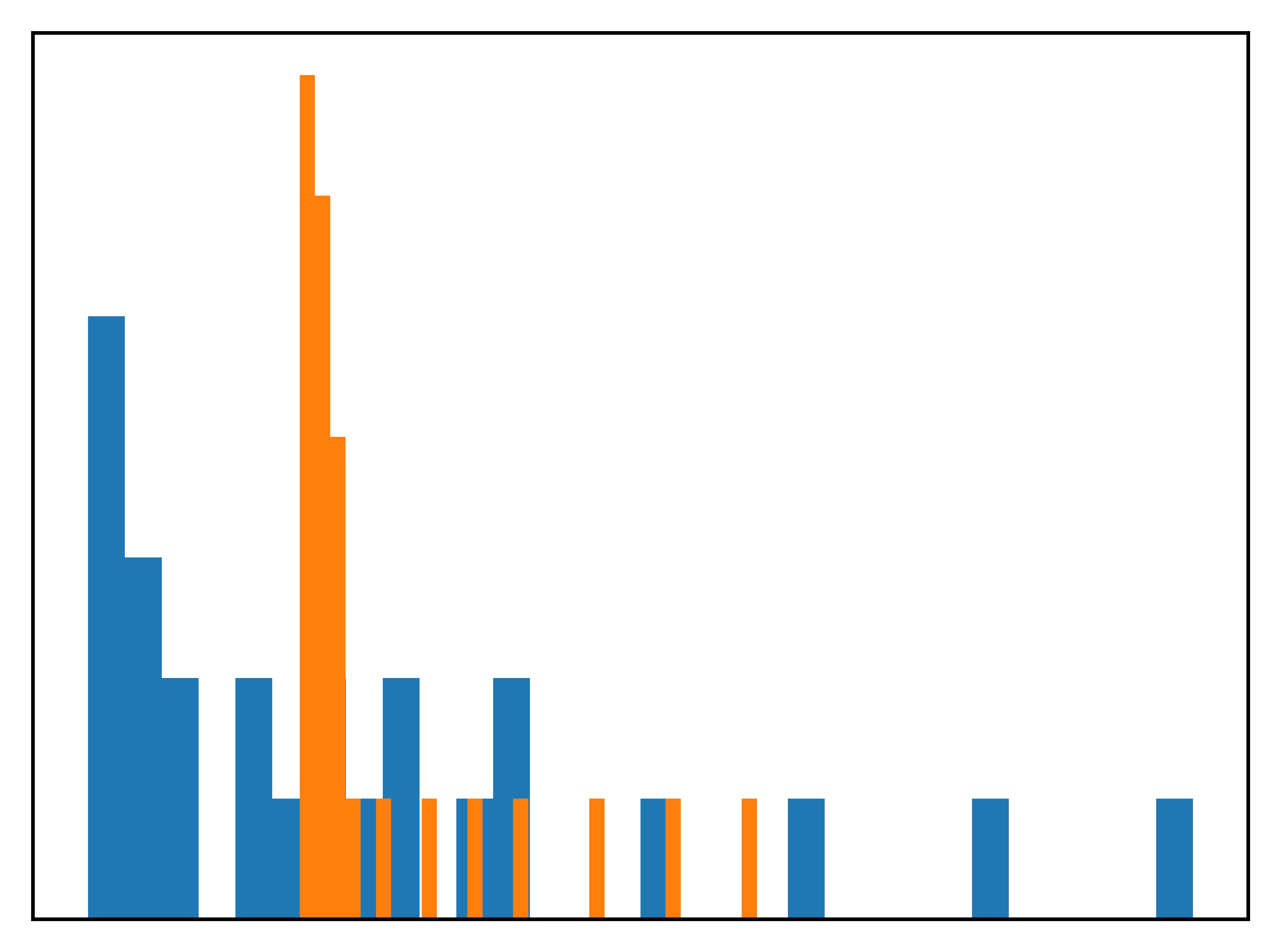

fig, ax = plt.subplots(figsize=(4, 3))

ax.errorbar(x, y2, yerr=y1, fmt="o-")

hide_labels(fig, ax)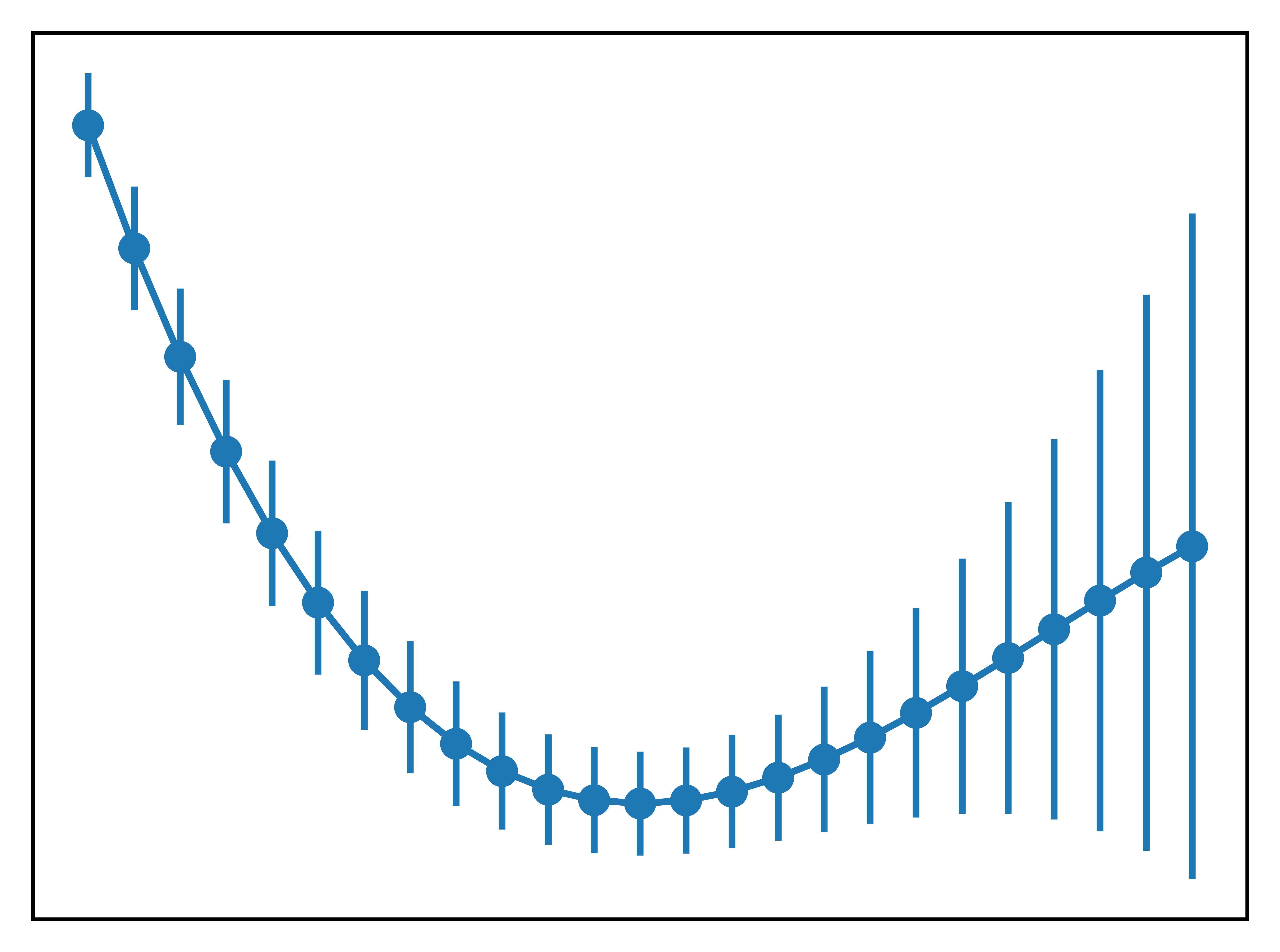

fig, ax = plt.subplots(figsize=(4, 3))

ax.stem(x, y2, "b", markerfmt="bs")
ax.stem(x, y1, "r", markerfmt="ro")

hide_labels(fig, ax)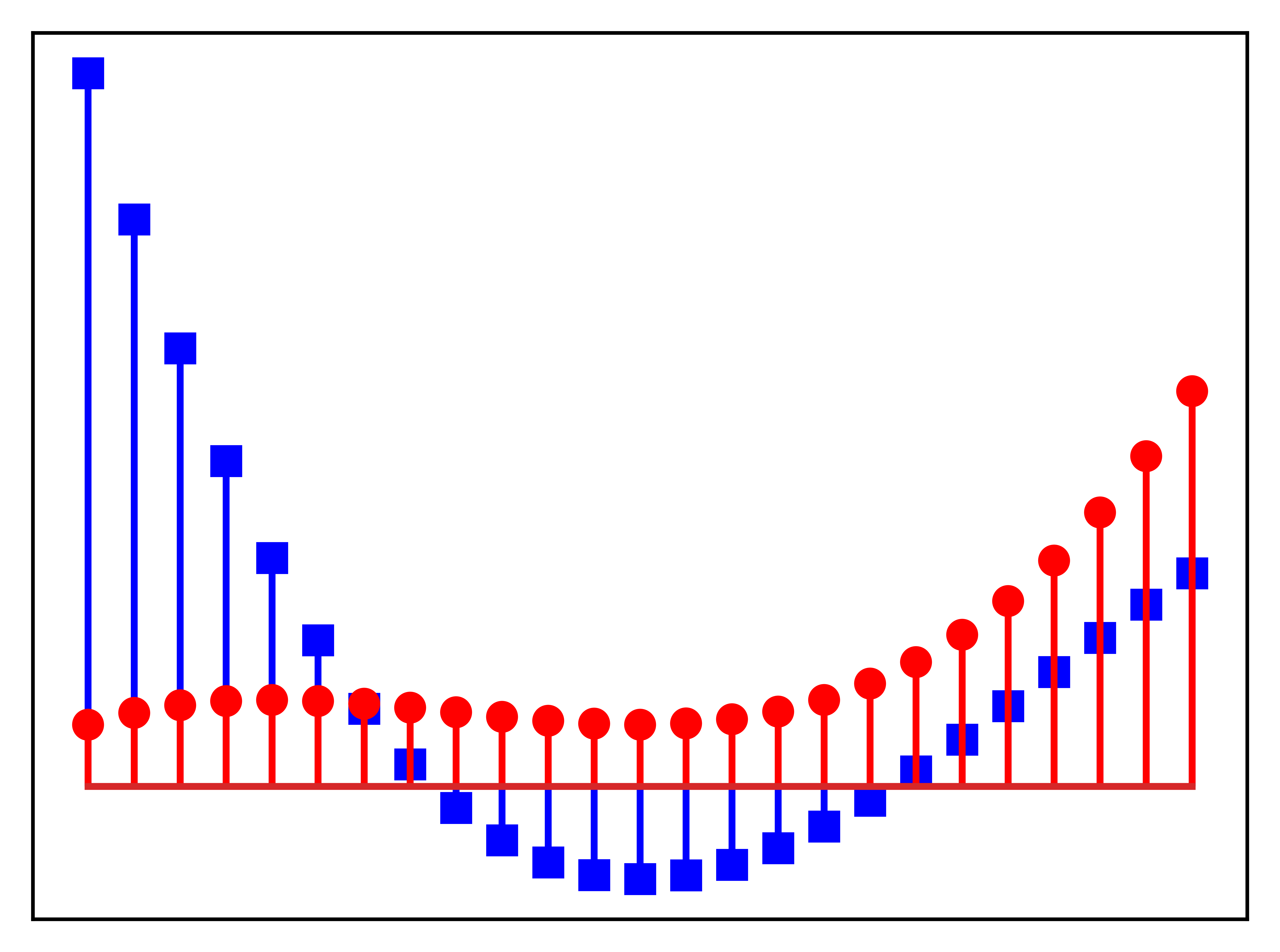

fig, ax = plt.subplots(figsize=(4, 3))

x = np.linspace(0, 5, 50)

ax.scatter(x, -1 + x + 0.25 * x**2 + 2 * np.random.rand(len(x)))
ax.scatter(x, np.sqrt(x) + 2 * np.random.rand(len(x)), color="green")

hide_labels(fig, ax)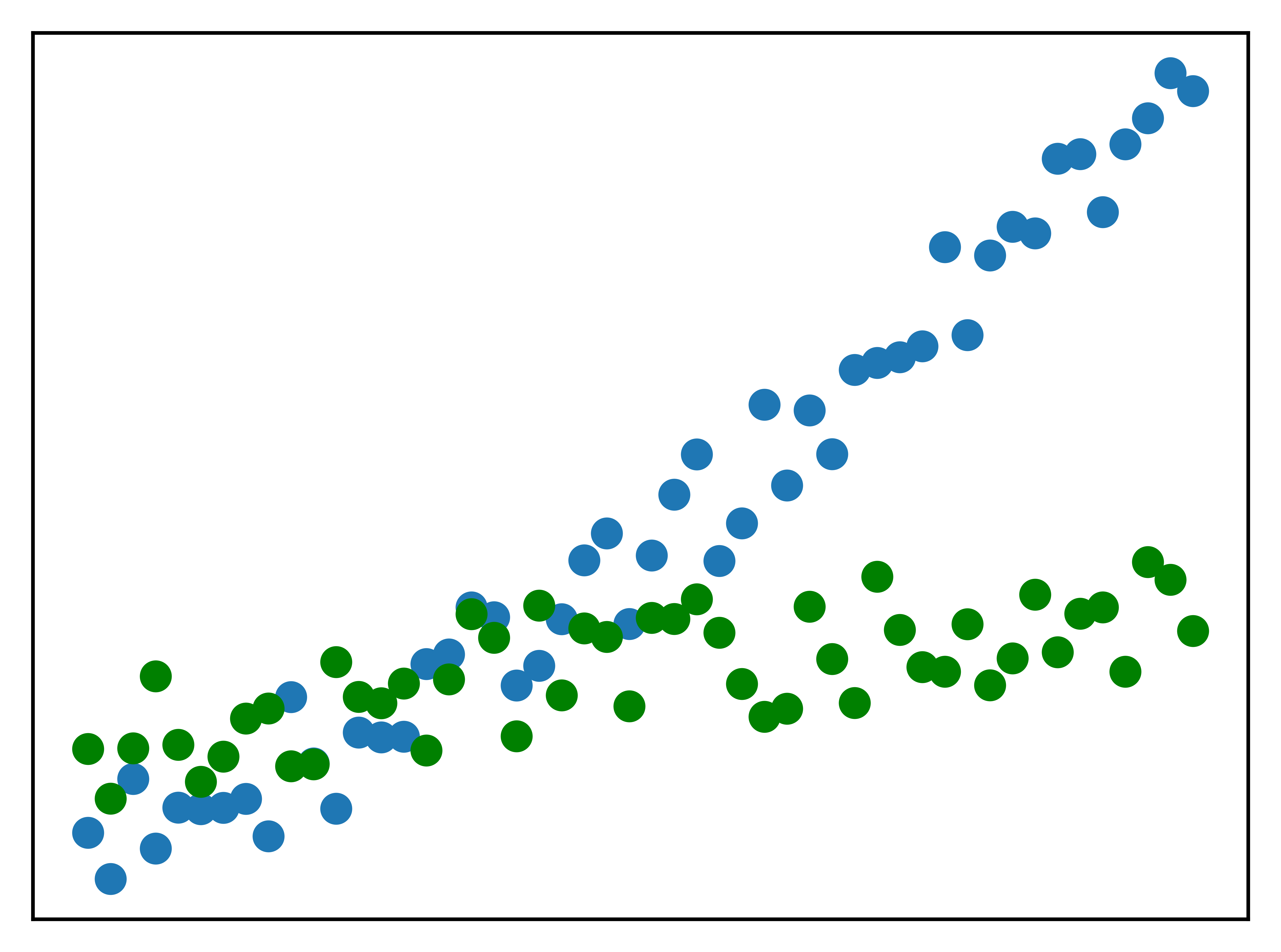

fig, ax = plt.subplots(figsize=(3, 3))

colors = ["yellowgreen", "gold", "lightskyblue", "lightcoral"]

x = y = np.linspace(-2, 2, 10)
X, Y = np.meshgrid(x, y)
U = np.sin(X)
V = np.sin(Y)

ax.quiver(X, Y, U, V)

hide_labels(fig, ax)

fig, ax = plt.subplots(figsize=(8, 4))

x = np.linspace(-20, 20, 100)
y = np.sin(x) / x

ax.plot(x, y)

ax.set_ylabel("y label")
ax.set_xlabel("x label")

for label in ax.get_xticklabels() + ax.get_yticklabels():
    label.set_rotation(45)

fig, ax = plt.subplots(figsize=(12, 3))

ax.set_yticks([])
ax.set_xticks([])
ax.set_xlim(-0.5, 3.5)
ax.set_ylim(-0.05, 0.25)
ax.axhline(0)

ax.text(0, 0.1, "Text label", fontsize=14, family="serif")

ax.plot(1, 0, "o")
ax.annotate(
    "Annotation",
    fontsize=14,
    family="serif",
    xy=(1, 0),
    xycoords="data",
    xytext=(+20, +50),
    textcoords="offset points",
    arrowprops=dict(arrowstyle="->", connectionstyle="arc3, rad=.5"),
)

ax.text(
    2,
    0.1,
    r"Equation: $i\hbar\partial_t \Psi = \hat{H}\Psi$",
    fontsize=14,
    family="serif",
)

fig.savefig("ch4-text-annotation.pdf")

fig, axes = plt.subplots(ncols=2, nrows=3)

x = np.linspace(-5, 5, 5)
y = np.ones_like(x)


def axes_settings(fig, ax, title, ymax):
    ax.set_xticks([])
    ax.set_yticks([])
    ax.set_ylim(0, ymax + 1)
    ax.set_title(title)


fig, axes = plt.subplots(1, 4, figsize=(16, 3))

# Line width
linewidths = [0.5, 1.0, 2.0, 4.0]
for n, linewidth in enumerate(linewidths):
    axes[0].plot(x, y + n, color="blue", linewidth=linewidth)
axes_settings(fig, axes[0], "linewidth", len(linewidths))

# Line style
linestyles = ["-", "-.", ":"]
for n, linestyle in enumerate(linestyles):
    axes[1].plot(x, y + n, color="blue", lw=2, linestyle=linestyle)

# custom dash style
(line,) = axes[1].plot(x, y + 3, color="blue", lw=2)
length1, gap1, length2, gap2 = 10, 7, 20, 7
line.set_dashes([length1, gap1, length2, gap2])
axes_settings(fig, axes[1], "linetypes", len(linestyles) + 1)

# marker types
markers = ["+", "o", "*", "s", ".", "1", "2", "3", "4"]
for n, marker in enumerate(markers):
    # lw = shorthand for linewidth, ls = shorthand for linestyle
    axes[2].plot(x, y + n, color="blue", lw=2, ls="None", marker=marker)
axes_settings(fig, axes[2], "markers", len(markers))


# marker size and color
markersizecolors = [(4, "white"), (8, "red"), (12, "yellow"), (16, "lightgreen")]
for n, (markersize, markerfacecolor) in enumerate(markersizecolors):
    axes[3].plot(
        x,
        y + n,
        color="blue",
        lw=1,
        ls="-",
        marker="o",
        markersize=markersize,
        markerfacecolor=markerfacecolor,
        markeredgewidth=2,
    )

axes_settings(fig, axes[3], "marker size/color", len(markersizecolors))

fig.savefig("ch4-line-styles.pdf")

import numpy as np
import sympy as s

# a symbolic variable for x, and a numerical array with specific values of x
sym_x = s.Symbol("x")
x = np.linspace(-2 * np.pi, 2 * np.pi, 100)


def sin_expansion(x, n):
    """
    Evaluate the nth order Talyor series expansion
    of sin(x) for the numerical values in the array x.
    """
    return s.lambdify(sym_x, s.sin(sym_x).series(n=n + 1).removeO(), "numpy")(x)


fig, ax = plt.subplots(figsize=(10, 6))

ax.plot(x, np.sin(x), linewidth=4, color="red", label="sin(x)")

colors = ["blue", "black"]
linestyles = [":", "-.", "--"]
for idx, n in enumerate(range(1, 12, 2)):
    ax.plot(
        x,
        sin_expansion(x, n),
        color=colors[idx // 3],
        linestyle=linestyles[idx % 3],
        linewidth=3,
        label="O(%d) approx." % (n + 1),
    )

ax.set_ylim(-1.1, 1.1)
ax.set_xlim(-1.5 * np.pi, 1.5 * np.pi)
ax.legend(bbox_to_anchor=(1.02, 1), loc=2, borderaxespad=0.0)
fig.subplots_adjust(right=0.75);

fig.savefig("ch4-sin-expansion.pdf")

fig, axes = plt.subplots(1, 2, figsize=(8, 3.5), sharey=True)

data1 = np.random.randn(200, 2) * np.array([3, 1])
area1 = (np.random.randn(200) + 0.5) * 100

data2 = np.random.randn(200, 2) * np.array([1, 3])
area2 = (np.random.randn(200) + 0.5) * 100

axes[0].scatter(data1[:, 0], data1[:, 1], color="green", marker="s", s=30, alpha=0.5)
axes[0].scatter(data2[:, 0], data2[:, 1], color="blue", marker="o", s=30, alpha=0.5)

axes[1].hist(
    [data1[:, 1], data2[:, 1]],
    bins=15,
    color=["green", "blue"],
    alpha=0.5,
    orientation="horizontal",
);

fig, axes = plt.subplots(1, 4, figsize=(16, 4))

x = np.linspace(0, 1, 100)

for n in range(4):
    axes[n].plot(x, x, label="y(x) = x")
    axes[n].plot(x, x + x**2, label="y(x) = x + x**2")
    axes[n].legend(loc=n + 1)
    axes[n].set_title("legend(loc=%d)" % (n + 1))

fig.tight_layout()
fig.savefig("ch4-legend-loc.pdf")

fig, ax = plt.subplots(1, 1, figsize=(8.5, 3))

x = np.linspace(-1, 1, 100)

for n in range(1, 9):
    ax.plot(x, n * x, label="y(x) = %d*x" % n)

ax.legend(ncol=4, loc=3, bbox_to_anchor=(0, 1), fontsize=12)
fig.subplots_adjust(top=0.75)
fig.savefig("ch4-legend-loc-2.pdf")

fig, ax = plt.subplots(figsize=(8, 3), subplot_kw={"facecolor": "#ebf5ff"})

x = np.linspace(0, 50, 500)
ax.plot(x, np.sin(x) * np.exp(-x / 10), lw=2)

ax.set_xlabel("x", labelpad=5, fontsize=18, fontname="serif", color="blue")
ax.set_ylabel("f(x)", labelpad=15, fontsize=18, fontname="serif", color="blue")
ax.set_title(
    "axis labels and title example",
    loc="left",
    fontsize=16,
    fontname="serif",
    color="blue",
)

fig.tight_layout()
fig.savefig("ch4-axis-labels.pdf")

x = np.linspace(0, 30, 500)
y = np.sin(x) * np.exp(-x / 10)

fig, axes = plt.subplots(1, 3, figsize=(11, 3), subplot_kw={"facecolor": "#ebf5ff"})

axes[0].plot(x, y, lw=2)
axes[0].set_xlim(-5, 35)
axes[0].set_ylim(-1, 1)
axes[0].set_title("set_xlim / set_y_lim")

axes[1].plot(x, y, lw=2)
axes[1].axis("tight")
axes[1].set_title("axis('tight')")

axes[2].plot(x, y, lw=2)
axes[2].axis("equal")
axes[2].set_title("axis('equal')")

fig.subplots_adjust(wspace=0.25)
fig.savefig("ch4-axis-ranges.pdf")

x = np.linspace(-2 * np.pi, 2 * np.pi, 500)
y = np.sin(x) * np.exp(-(x**2) / 20)

fig, axes = plt.subplots(1, 4, figsize=(12, 3))

axes[0].plot(x, y, lw=2)
axes[0].set_title("default ticks")

axes[1].plot(x, y, lw=2)
axes[1].set_yticks([-1, 0, 1])
axes[1].set_xticks([-5, 0, 5])
axes[1].set_title("set_xticks")

axes[2].plot(x, y, lw=2)
axes[2].xaxis.set_major_locator(mpl.ticker.MaxNLocator(4))
axes[2].yaxis.set_major_locator(mpl.ticker.FixedLocator([-1, 0, 1]))
axes[2].xaxis.set_minor_locator(mpl.ticker.MaxNLocator(8))
axes[2].yaxis.set_minor_locator(mpl.ticker.MaxNLocator(8))
axes[2].set_title("set_major_locator")

axes[3].plot(x, y, lw=2)
axes[3].set_yticks([-1, 0, 1])
axes[3].set_xticks([-2 * np.pi, -np.pi, 0, np.pi, 2 * np.pi])
axes[3].set_xticklabels(["$-2\pi$", "$-\pi$", 0, r"$\pi$", r"$2\pi$"])
axes[3].xaxis.set_minor_locator(
    mpl.ticker.FixedLocator([-3 * np.pi / 2, -np.pi / 2, 0, np.pi / 2, 3 * np.pi / 2])
)
axes[3].yaxis.set_minor_locator(mpl.ticker.MaxNLocator(4))
axes[3].set_title("set_xticklabels")

fig.tight_layout()
fig.savefig("ch4-axis-ticks.pdf")

fig, axes = plt.subplots(1, 3, figsize=(12, 4))

x_major_ticker = mpl.ticker.MultipleLocator(4)
x_minor_ticker = mpl.ticker.MultipleLocator(1)
y_major_ticker = mpl.ticker.MultipleLocator(0.5)
y_minor_ticker = mpl.ticker.MultipleLocator(0.25)

for ax in axes:
    ax.plot(x, y, lw=2)
    ax.xaxis.set_major_locator(x_major_ticker)
    ax.yaxis.set_major_locator(y_major_ticker)
    ax.xaxis.set_minor_locator(x_minor_ticker)
    ax.yaxis.set_minor_locator(y_minor_ticker)

axes[0].set_title("default grid")
axes[0].grid()

axes[1].set_title("major/minor grid")
axes[1].grid(color="blue", which="both", linestyle=":", linewidth=0.5)

axes[2].set_title("individual x/y major/minor grid")
axes[2].grid(color="grey", which="major", axis="x", linestyle="-", linewidth=0.5)
axes[2].grid(color="grey", which="minor", axis="x", linestyle=":", linewidth=0.25)
axes[2].grid(color="grey", which="major", axis="y", linestyle="-", linewidth=0.5)

fig.tight_layout()
fig.savefig("ch4-axis-grid.pdf")

fig, axes = plt.subplots(1, 2, figsize=(8, 3))

x = np.linspace(0, 1e5, 100)
y = x**2

axes[0].plot(x, y, "b.")
axes[0].set_title("default labels", loc="right")

axes[1].plot(x, y, "b")
axes[1].set_title("scientific notation labels", loc="right")

formatter = mpl.ticker.ScalarFormatter(useMathText=True)
formatter.set_scientific(True)
formatter.set_powerlimits((-1, 1))
axes[1].xaxis.set_major_formatter(formatter)
axes[1].yaxis.set_major_formatter(formatter)

fig.tight_layout()
fig.savefig("ch4-axis-scientific.pdf")

fig, axes = plt.subplots(1, 3, figsize=(12, 3))

x = np.linspace(0, 1e3, 100)
y1, y2 = x**3, x**4

axes[0].set_title("loglog")
axes[0].loglog(x, y1, "b", x, y2, "r")

axes[1].set_title("semilogy")
axes[1].semilogy(x, y1, "b", x, y2, "r")

axes[2].set_title("plot / set_xscale / set_yscale")
axes[2].plot(x, y1, "b", x, y2, "r")
axes[2].set_xscale("log")
axes[2].set_yscale("log")

fig.tight_layout()
fig.savefig("ch4-axis-log-plots.pdf")

fig, ax1 = plt.subplots(figsize=(8, 4))

r = np.linspace(0, 5, 100)
a = 4 * np.pi * r**2  # area
v = (4 * np.pi / 3) * r**3  # volume


ax1.set_title("surface area and volume of a sphere", fontsize=16)
ax1.set_xlabel("radius [m]", fontsize=16)

ax1.plot(r, a, lw=2, color="blue")
ax1.set_ylabel(r"surface area ($m^2$)", fontsize=16, color="blue")
for label in ax1.get_yticklabels():
    label.set_color("blue")

ax2 = ax1.twinx()
ax2.plot(r, v, lw=2, color="red")
ax2.set_ylabel(r"volume ($m^3$)", fontsize=16, color="red")
for label in ax2.get_yticklabels():
    label.set_color("red")

fig.tight_layout()
fig.savefig("ch4-axis-twin-ax.pdf")

x = np.linspace(-10, 10, 500)
y = np.sin(x) / x

fig, ax = plt.subplots(figsize=(8, 4))

ax.plot(x, y, linewidth=2)

# remove top and right spines
ax.spines["right"].set_color("none")
ax.spines["top"].set_color("none")

# remove top and right spine ticks
ax.xaxis.set_ticks_position("bottom")
ax.yaxis.set_ticks_position("left")

# move bottom and left spine to x = 0 and y = 0
ax.spines["bottom"].set_position(("data", 0))
ax.spines["left"].set_position(("data", 0))

ax.set_xticks([-10, -5, 5, 10])
ax.set_yticks([0.5, 1])

# give each label a solid background of white, to not overlap with the plot line
for label in ax.get_xticklabels() + ax.get_yticklabels():
    label.set_bbox({"facecolor": "white", "edgecolor": "white"})

fig.tight_layout()
fig.savefig("ch4-axis-spines.pdf")

fig = plt.figure(figsize=(8, 4))


def f(x):
    return 1 / (1 + x**2) + 0.1 / (1 + ((3 - x) / 0.1) ** 2)


def plot_and_format_axes(ax, x, f, fontsize):
    ax.plot(x, f(x), linewidth=2)
    ax.xaxis.set_major_locator(mpl.ticker.MaxNLocator(5))
    ax.yaxis.set_major_locator(mpl.ticker.MaxNLocator(4))
    ax.set_xlabel(r"$x$", fontsize=fontsize)
    ax.set_ylabel(r"$f(x)$", fontsize=fontsize)


# main graph
ax = fig.add_axes([0.1, 0.15, 0.8, 0.8], facecolor="#f5f5f5")
x = np.linspace(-4, 14, 1000)
plot_and_format_axes(ax, x, f, 18)

# inset
x0, x1 = 2.5, 3.5
ax.axvline(x0, ymax=0.3, color="grey", linestyle=":")
ax.axvline(x1, ymax=0.3, color="grey", linestyle=":")

ax = fig.add_axes([0.5, 0.5, 0.38, 0.42], facecolor="none")
x = np.linspace(x0, x1, 1000)
plot_and_format_axes(ax, x, f, 14)

fig.savefig("ch4-advanced-axes-inset.pdf")

ncols, nrows = 3, 3

fig, axes = plt.subplots(nrows, ncols)

for m in range(nrows):
    for n in range(ncols):
        axes[m, n].set_xticks([])
        axes[m, n].set_yticks([])
        axes[m, n].text(0.5, 0.5, "axes[%d, %d]" % (m, n), horizontalalignment="center")

fig, axes = plt.subplots(2, 2, figsize=(6, 6), sharex=True, sharey=True, squeeze=False)

x1 = np.random.randn(100)
x2 = np.random.randn(100)

axes[0, 0].set_title("Uncorrelated")
axes[0, 0].scatter(x1, x2)

axes[0, 1].set_title("Weakly positively correlated")
axes[0, 1].scatter(x1, x1 + x2)

axes[1, 0].set_title("Weakly negatively correlated")
axes[1, 0].scatter(x1, -x1 + x2)

axes[1, 1].set_title("Strongly correlated")
axes[1, 1].scatter(x1, x1 + 0.15 * x2)

axes[1, 1].set_xlabel("x")
axes[1, 0].set_xlabel("x")
axes[0, 0].set_ylabel("y")
axes[1, 0].set_ylabel("y")

plt.subplots_adjust(left=0.1, right=0.95, bottom=0.1, top=0.95, wspace=0.1, hspace=0.2)

fig.savefig("ch4-advanced-axes-subplots.pdf")

fig = plt.figure()


def clear_ticklabels(ax):
    ax.set_yticklabels([])
    ax.set_xticklabels([])


ax0 = plt.subplot2grid((3, 3), (0, 0))
ax1 = plt.subplot2grid((3, 3), (0, 1))
ax2 = plt.subplot2grid((3, 3), (1, 0), colspan=2)
ax3 = plt.subplot2grid((3, 3), (2, 0), colspan=3)
ax4 = plt.subplot2grid((3, 3), (0, 2), rowspan=2)

axes = [ax0, ax1, ax2, ax3, ax4]
[
    ax.text(0.5, 0.5, "ax%d" % n, horizontalalignment="center")
    for n, ax in enumerate(axes)
]
[clear_ticklabels(ax) for ax in axes]

fig.savefig("ch4-advanced-axes-subplot2grid.pdf")

from matplotlib.gridspec import GridSpec

fig = plt.figure(figsize=(6, 4))

gs = mpl.gridspec.GridSpec(4, 4)

ax0 = fig.add_subplot(gs[0, 0])
ax1 = fig.add_subplot(gs[1, 1])
ax2 = fig.add_subplot(gs[2, 2])
ax3 = fig.add_subplot(gs[3, 3])

ax4 = fig.add_subplot(gs[0, 1:])
ax5 = fig.add_subplot(gs[1:, 0])

ax6 = fig.add_subplot(gs[1, 2:])
ax7 = fig.add_subplot(gs[2:, 1])

ax8 = fig.add_subplot(gs[2, 3])
ax9 = fig.add_subplot(gs[3, 2])


def clear_ticklabels(ax):
    ax.set_yticklabels([])
    ax.set_xticklabels([])


axes = [ax0, ax1, ax2, ax3, ax4, ax5, ax6, ax7, ax8, ax9]
[
    ax.text(0.5, 0.5, "ax%d" % n, horizontalalignment="center")
    for n, ax in enumerate(axes)
]
[clear_ticklabels(ax) for ax in axes]

fig.savefig("ch4-advanced-axes-gridspec-1.pdf")

fig = plt.figure(figsize=(4, 4))

gs = mpl.gridspec.GridSpec(
    2, 2, width_ratios=[4, 1], height_ratios=[1, 4], wspace=0.05, hspace=0.05
)

ax0 = fig.add_subplot(gs[1, 0])
ax1 = fig.add_subplot(gs[0, 0])
ax2 = fig.add_subplot(gs[1, 1])


def clear_ticklabels(ax):
    ax.set_yticklabels([])
    ax.set_xticklabels([])


axes = [ax0, ax1, ax2]
[
    ax.text(0.5, 0.5, "ax%d" % n, horizontalalignment="center")
    for n, ax in enumerate(axes)
]
[clear_ticklabels(ax) for ax in axes]

fig.savefig("ch4-advanced-axes-gridspec-2.pdf")

x = y = np.linspace(-2, 2, 150)
X, Y = np.meshgrid(x, y)

R1 = np.sqrt((X + 0.5) ** 2 + (Y + 0.5) ** 2)
R2 = np.sqrt((X + 0.5) ** 2 + (Y - 0.5) ** 2)
R3 = np.sqrt((X - 0.5) ** 2 + (Y + 0.5) ** 2)
R4 = np.sqrt((X - 0.5) ** 2 + (Y - 0.5) ** 2)

Z = np.sin(10 * R1) / (10 * R1) + np.sin(20 * R4) / (20 * R4)

fig, ax = plt.subplots(figsize=(6, 5))

p = ax.pcolor(X, Y, Z, cmap="seismic", vmin=-abs(Z).max(), vmax=abs(Z).max())
ax.axis("tight")
ax.set_xlabel("x")
ax.set_ylabel("y")
cb = fig.colorbar(p, ax=ax)

Z = 1 / R1 - 1 / R2 - 1 / R3 + 1 / R4

fig, ax = plt.subplots(figsize=(6, 5))

im = ax.imshow(
    Z, vmin=-1, vmax=1, cmap=mpl.cm.bwr, extent=[x.min(), x.max(), y.min(), y.max()]
)
im.set_interpolation("bilinear")

ax.axis("tight")
ax.set_xlabel("x")
ax.set_ylabel("y")
cb = fig.colorbar(p, ax=ax)

x = y = np.linspace(-2, 2, 150)
X, Y = np.meshgrid(x, y)

R1 = np.sqrt((X + 0.5) ** 2 + (Y + 0.5) ** 2)
R2 = np.sqrt((X + 0.5) ** 2 + (Y - 0.5) ** 2)
R3 = np.sqrt((X - 0.5) ** 2 + (Y + 0.5) ** 2)
R4 = np.sqrt((X - 0.5) ** 2 + (Y - 0.5) ** 2)

fig, axes = plt.subplots(1, 4, figsize=(14, 3))

Z = np.sin(10 * R1) / (10 * R1) + np.sin(20 * R4) / (20 * R4)


p = axes[0].pcolor(X, Y, Z, cmap="seismic", vmin=-abs(Z).max(), vmax=abs(Z).max())
axes[0].axis("tight")
axes[0].set_xlabel("x")
axes[0].set_ylabel("y")
axes[0].set_title("pcolor")
axes[0].xaxis.set_major_locator(mpl.ticker.MaxNLocator(4))
axes[0].yaxis.set_major_locator(mpl.ticker.MaxNLocator(4))


cb = fig.colorbar(p, ax=axes[0])
cb.set_label("z")
cb.set_ticks([-1, -0.5, 0, 0.5, 1])


Z = 1 / R1 - 1 / R2 - 1 / R3 + 1 / R4

im = axes[1].imshow(
    Z, vmin=-1, vmax=1, cmap=mpl.cm.bwr, extent=[x.min(), x.max(), y.min(), y.max()]
)
im.set_interpolation("bilinear")

axes[1].axis("tight")
axes[1].set_xlabel("x")
axes[1].set_ylabel("y")
axes[1].set_title("imshow")
cb = fig.colorbar(im, ax=axes[1])

axes[1].xaxis.set_major_locator(mpl.ticker.MaxNLocator(4))
axes[1].yaxis.set_major_locator(mpl.ticker.MaxNLocator(4))
# cb.ax.set_axes_locator(mpl.ticker.MaxNLocator(4))
cb.set_label("z")
cb.set_ticks([-1, -0.5, 0, 0.5, 1])

x = y = np.linspace(0, 1, 75)
X, Y = np.meshgrid(x, y)
Z = -2 * np.cos(2 * np.pi * X) * np.cos(2 * np.pi * Y) - 0.7 * np.cos(
    np.pi - 4 * np.pi * X
)

c = axes[2].contour(X, Y, Z, 15, cmap=mpl.cm.RdBu, vmin=-1, vmax=1)

axes[2].axis("tight")
axes[2].set_xlabel("x")
axes[2].set_ylabel("y")
axes[2].set_title("contour")

axes[2].xaxis.set_major_locator(mpl.ticker.MaxNLocator(4))
axes[2].yaxis.set_major_locator(mpl.ticker.MaxNLocator(4))


c = axes[3].contourf(X, Y, Z, 15, cmap=mpl.cm.RdBu, vmin=-1, vmax=1)

axes[3].axis("tight")
axes[3].set_xlabel("x")
axes[3].set_ylabel("y")
axes[3].set_title("contourf")

axes[3].xaxis.set_major_locator(mpl.ticker.MaxNLocator(4))
axes[3].yaxis.set_major_locator(mpl.ticker.MaxNLocator(4))

fig.tight_layout()
fig.savefig("ch4-colormaps.pdf")

fig, ax = plt.subplots(figsize=(6, 5))

x = y = np.linspace(0, 1, 75)
X, Y = np.meshgrid(x, y)

Z = -2 * np.cos(2 * np.pi * X) * np.cos(2 * np.pi * Y) - 0.7 * np.cos(
    np.pi - 4 * np.pi * X
)

c = ax.contour(X, Y, Z, 15, cmap=mpl.cm.RdBu, vmin=-1, vmax=1)

ax.axis("tight")
ax.set_xlabel("x")
ax.set_ylabel("y")

x = y = np.linspace(-10, 10, 150)
X, Y = np.meshgrid(x, y)
Z = np.cos(X) * np.cos(Y) * np.exp(-((X / 5) ** 2) - (Y / 5) ** 2)

fig, ax = plt.subplots(figsize=(6, 5))

p = ax.pcolor(X, Y, Z, vmin=-abs(Z).max(), vmax=abs(Z).max(), cmap=mpl.cm.bwr)

ax.axis("tight")
ax.set_xlabel(r"$x$", fontsize=18)
ax.set_ylabel(r"$y$", fontsize=18)
ax.xaxis.set_major_locator(mpl.ticker.MaxNLocator(4))
ax.yaxis.set_major_locator(mpl.ticker.MaxNLocator(4))

cb = fig.colorbar(p, ax=ax)
cb.set_label(r"$z$", fontsize=18)
cb.set_ticks([-1, -0.5, 0, 0.5, 1])

fig.savefig("ch4-colormap-pcolor.pdf")

from mpl_toolkits.mplot3d.axes3d import Axes3D

x = y = np.linspace(-3, 3, 74)
X, Y = np.meshgrid(x, y)

R = np.sqrt(X**2 + Y**2)
Z = np.sin(4 * R) / R

fig, axes = plt.subplots(1, 3, figsize=(14, 4), subplot_kw={"projection": "3d"})


def title_and_labels(ax, title):
    ax.set_title(title)
    ax.set_xlabel("$x$", fontsize=16)
    ax.set_ylabel("$y$", fontsize=16)
    ax.set_zlabel("$z$", fontsize=16)


norm = mpl.colors.Normalize(-abs(Z).max(), abs(Z).max())

p = axes[0].plot_surface(
    X,
    Y,
    Z,
    rstride=1,
    cstride=1,
    linewidth=0,
    antialiased=False,
    norm=norm,
    cmap=mpl.cm.Blues,
)
cb = fig.colorbar(p, ax=axes[0], shrink=0.6)
title_and_labels(axes[0], "plot_surface")

p = axes[1].plot_wireframe(X, Y, Z, rstride=2, cstride=2, color="darkgrey")
title_and_labels(axes[1], "plot_wireframe")

cset = axes[2].contour(X, Y, Z, zdir="z", offset=0, norm=norm, cmap=mpl.cm.Blues)
cset = axes[2].contour(X, Y, Z, zdir="y", offset=3, norm=norm, cmap=mpl.cm.Blues)
title_and_labels(axes[2], "contour")

fig.tight_layout()
fig.savefig("ch4-3d-plots-1.png", dpi=200)

fig, axes = plt.subplots(1, 3, figsize=(14, 4), subplot_kw={"projection": "3d"})


def title_and_labels(ax, title):
    ax.set_title(title)
    ax.set_xlabel("$x$", fontsize=16)
    ax.set_ylabel("$y$", fontsize=16)
    ax.set_zlabel("$z$", fontsize=16)


norm = mpl.colors.Normalize(-abs(Z).max(), abs(Z).max())

r = np.linspace(0, 10, 100)
p = axes[0].plot(np.cos(r), np.sin(r), 6 - r)
# cb = fig.colorbar(p, ax=axes[0], shrink=0.6)
title_and_labels(axes[0], "plot")

p = axes[1].scatter(np.cos(r), np.sin(r), 6 - r)
title_and_labels(axes[1], "scatter")

r = np.linspace(0, 6, 20)
p = axes[2].bar3d(
    np.cos(r),
    np.sin(r),
    0 * np.ones_like(r),
    0.05 * np.ones_like(r),
    0.05 * np.ones_like(r),
    6 - r,
)
title_and_labels(axes[2], "contour")
axes[2].text(0, 0, 0, "label")
fig.tight_layout()
fig.savefig("ch4-3d-plots-2.png", dpi=200)