First import the most important modules
import time

import matplotlib.pyplot as plt
import numpy as np
# import pandas as pd
# pd.set_option("display.max_columns", None)
# pd.set_option("display.width", None)
# pd.set_option("display.max_rows", None)
# pd.DataFrame(A)Numpy arrays
The main advantage of numpy is arrays. It’s a way to add /subtract/multiply/... many numbers in one line.
Creation of arrays
There are many ways to create arrays, the most important one are listed below
# create numpy array from a python list
a = np.array([1, 2, 3])
print(a)
print(type(a))

# create numpy array with zeros
b = np.zeros(5)
print(b)

# create numpy array with equal spacing
c = np.linspace(0, 10, 5)  # start stop steps
print(c)
# or
c = np.arange(0, 10, 2)  # start stop stepzise
print(c)
[1 2 3]
<class 'numpy.ndarray'>
[0. 0. 0. 0. 0.]
[ 0. 2.5 5. 7.5 10. ]
[0 2 4 6 8]
More dimensional arrays are possible, too.
# create 2d array
d = np.array([[1, 2, 3], [4, 5, 6], [7, 8, 9]])
print(d)
print(d.shape)  # shows the dimensions of the array

# or 2d zeros
e = np.zeros((3, 3))
print(e)
[[1 2 3]
[4 5 6]
[7 8 9]]
(3, 3)
[[0. 0. 0.]
[0. 0. 0.]
[0. 0. 0.]]
Access and slicing
Of course, we will modify the entries of an array.
a = np.array([1, 2, 3])
print("before", a)
a[0] = 10  # acces first element and set it to 10
print("after", a)
print("last element", a[-1])


b = np.array([[1, 2, 3], [4, 5, 6], [7, 8, 9]])
print("\nentries of array:", b[0, 1])  # access first row, second column
before [1 2 3]
after [10 2 3]
last element 3
entries of array: 2
A nice feature is the access of ranges via “:”
barray([[1, 2, 3],
[4, 5, 6],
[7, 8, 9]])print(a[1:2])
print(a[1:])
# or in more dimensions
print(b[:, 1]) # access all rows, second column
print(b[1, :]) # access second row, all columns[2]
[2 3]
[2 5 8]
[4 5 6]
Exercises
Create an array with time steps between 0, 0.01, 0.02, 0.03 ... 1
Print from this the numbers 0.5, 0.51,...,0.56
create a 3x3 array with the numbers from 1-9. (.reshape may help...)
print the second column, and the second row
change the number in the middle to 55
print the 2nd row and column again
Solution
a = np.arange(0, 1 + 0.01, 0.01)
print(a)
print(a[50:57])
[0. 0.01 0.02 0.03 0.04 0.05 0.06 0.07 0.08 0.09 0.1 0.11 0.12 0.13
0.14 0.15 0.16 0.17 0.18 0.19 0.2 0.21 0.22 0.23 0.24 0.25 0.26 0.27
0.28 0.29 0.3 0.31 0.32 0.33 0.34 0.35 0.36 0.37 0.38 0.39 0.4 0.41
0.42 0.43 0.44 0.45 0.46 0.47 0.48 0.49 0.5 0.51 0.52 0.53 0.54 0.55
0.56 0.57 0.58 0.59 0.6 0.61 0.62 0.63 0.64 0.65 0.66 0.67 0.68 0.69
0.7 0.71 0.72 0.73 0.74 0.75 0.76 0.77 0.78 0.79 0.8 0.81 0.82 0.83
0.84 0.85 0.86 0.87 0.88 0.89 0.9 0.91 0.92 0.93 0.94 0.95 0.96 0.97
0.98 0.99 1. ]
[0.5 0.51 0.52 0.53 0.54 0.55 0.56]
b = np.arange(1, 10).reshape(3, 3)
print(b)
print(b[:, 1])  # second column
print(b[1, :])  # second row
b[1, 1] = 55
print(b[:, 1])  # second column
print(b[1, :])  # second row
[[1 2 3]
[4 5 6]
[7 8 9]]
[2 5 8]
[4 5 6]
[ 2 55 8]
[ 4 55 6]
Basic arithmetics and functions
You can add, multiply, ... arrays like normal numbers, if
to a scalar
to an array of same size
a = np.linspace(0, 10, 5)
print("a", a)
b = 3 * a + 1
print("3a+1", b)
print("a^2-b", a**2 - b)
print("The sum of ", a, "is ", np.sum(a))
a [ 0. 2.5 5. 7.5 10. ]
3a+1 [ 1. 8.5 16. 23.5 31. ]
a^2-b [-1. -2.25 9. 32.75 69. ]
The sum of [ 0. 2.5 5. 7.5 10. ] is 25.0
Functions work as well:
times = np.linspace(0, 2 * np.pi, 100)
signal = np.sin(times)

plt.plot(times, signal, label="sin(t)")
plt.title("A wonderful plot")
plt.xlabel("t")
plt.ylabel("signal")
plt.legend()
plt.show()
Exercises
Calculate the scalar product of the vectors (1,2,3) and (3,2,1)
plot the functions and from -1 to 1
add a title and a legend to the plot
Solution
# this space is for your code
x = np.array([1, 2, 3])
y = np.array([3, 2, 1])
print(np.dot(x, y))
10
x = np.linspace(-1, 1)
plt.plot(x, x**2, label=r"$x^2$")
plt.plot(x, np.sqrt(x**2 + 1), label=r"$\sqrt{x^2+1}$")
plt.title("Plots")
plt.legend()
plt.show()
Vectors and matrices
Of course, we can use matrices and vectors as well.
# create a 5x5 identity matrix
A = np.eye(5)
print(A)
# modify the matrix
A[:, 3] = 1  # la cuarta columna de A es 1
print(A)
A[3, :] = -1  # la cuarta fila de A es 1
print(A)
# create a random vector
v = np.random.rand(5)
print(A)
print(v)
# calculate matrix vector multiplication A*v
w = A @ v
print(w)
# or in pictures
fig, ax = plt.subplots(1, 3, figsize=(15, 5))
im = ax[0].matshow(A)
ax[0].set_title("A")
ax[1].matshow(v.reshape(5, 1))  # matshow expects a 2d array
ax[1].set_title("v")
ax[2].matshow(w.reshape(5, 1))
ax[2].set_title("A*v")
fig.colorbar(im, ax=ax)
plt.show()
[[1. 0. 0. 0. 0.]
[0. 1. 0. 0. 0.]
[0. 0. 1. 0. 0.]
[0. 0. 0. 1. 0.]
[0. 0. 0. 0. 1.]]
[[1. 0. 0. 1. 0.]
[0. 1. 0. 1. 0.]
[0. 0. 1. 1. 0.]
[0. 0. 0. 1. 0.]
[0. 0. 0. 1. 1.]]
[[ 1. 0. 0. 1. 0.]
[ 0. 1. 0. 1. 0.]
[ 0. 0. 1. 1. 0.]
[-1. -1. -1. -1. -1.]
[ 0. 0. 0. 1. 1.]]
[[ 1. 0. 0. 1. 0.]
[ 0. 1. 0. 1. 0.]
[ 0. 0. 1. 1. 0.]
[-1. -1. -1. -1. -1.]
[ 0. 0. 0. 1. 1.]]
[0.35075525 0.55437656 0.45529011 0.96491082 0.52245486]
[ 1.31566607 1.51928739 1.42020093 -2.84778761 1.48736569]
/usr/lib/python3.13/site-packages/IPython/core/pylabtools.py:170: UserWarning: This figure includes Axes that are not compatible with tight_layout, so results might be incorrect.
  fig.canvas.print_figure(bytes_io, **kw)
?np.random.randSignature: np.random.rand(*args)
Docstring:
rand(d0, d1, ..., dn)
Random values in a given shape.
.. note::
This is a convenience function for users porting code from Matlab,
and wraps `random_sample`. That function takes a
tuple to specify the size of the output, which is consistent with
other NumPy functions like `numpy.zeros` and `numpy.ones`.
Create an array of the given shape and populate it with
random samples from a uniform distribution
over ``[0, 1)``.
Parameters
----------
d0, d1, ..., dn : int, optional
The dimensions of the returned array, must be non-negative.
If no argument is given a single Python float is returned.
Returns
-------
out : ndarray, shape ``(d0, d1, ..., dn)``
Random values.
See Also
--------
random
Examples
--------
>>> np.random.rand(3,2)
array([[ 0.14022471, 0.96360618], #random
[ 0.37601032, 0.25528411], #random
[ 0.49313049, 0.94909878]]) #random
Type: methodAnother handy function: np.diag
A = np.eye(5)
# returns the diagonal entries of matrix
print(np.diag(A))
v = np.random.rand(5)
print(v)

# or create matrices from a vector
fig, ax = plt.subplots(1, 2, figsize=(10, 5))
ax[0].matshow(np.diag(v))
im = ax[1].matshow(np.diag(v[:-1], k=1))
fig.colorbar(im, ax=ax)
[1. 1. 1. 1. 1.]
[0.60289977 0.45886676 0.69339036 0.49860322 0.85619674]
/usr/lib/python3.13/site-packages/IPython/core/events.py:82: UserWarning: This figure includes Axes that are not compatible with tight_layout, so results might be incorrect.
  func(*args, **kwargs)
Exercises
Create a random 5x5 Matrix
plot this matrix
Create tridiagonal matrix, which has 2 on its diagonal and -1 on both first off diagonals.
apply this matrix to the vector (0,0,1,0,0)
Solution
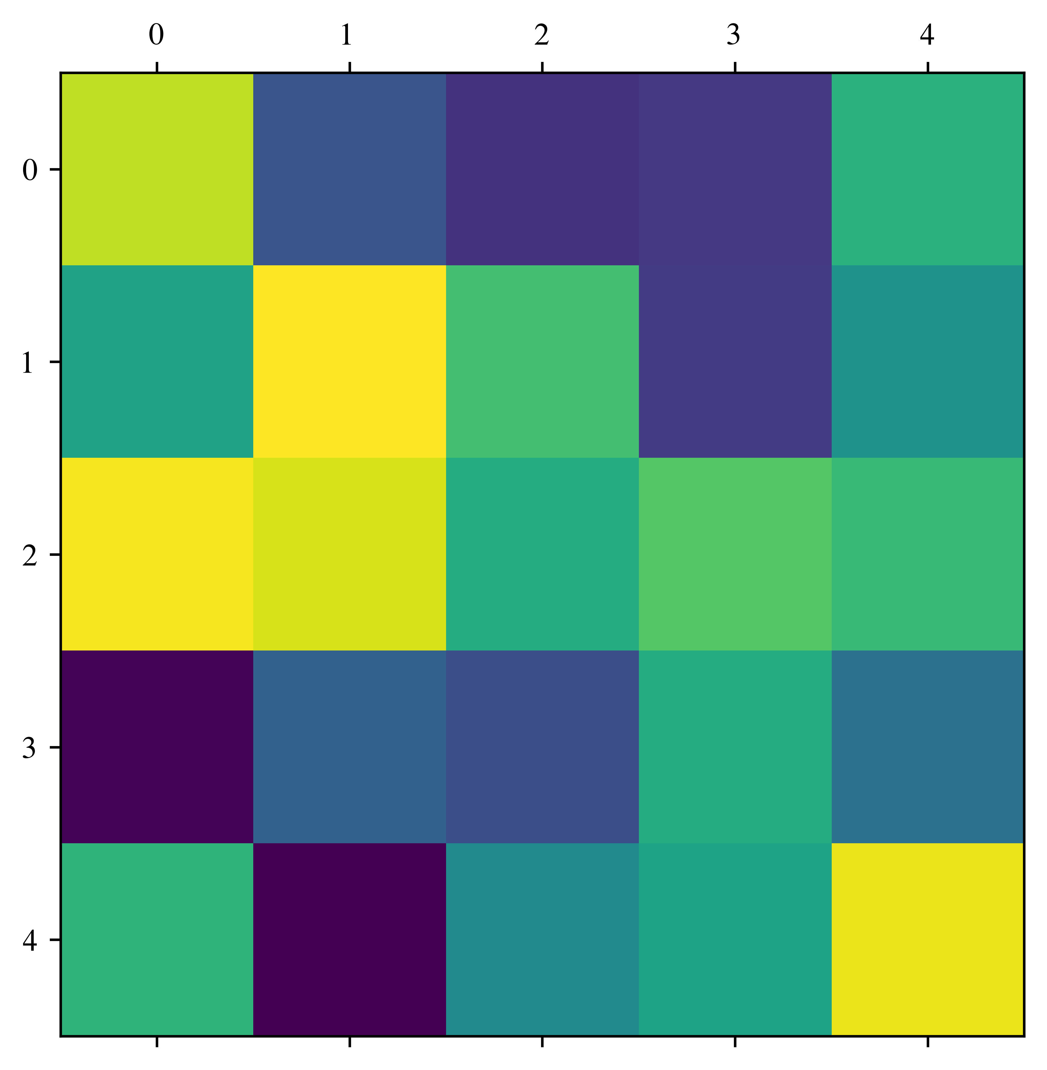
A = np.random.rand(5, 5)
print(A)
fig, ax = plt.subplots()
ax.matshow(A)
plt.show()
[[0.88784275 0.26270944 0.14751584 0.16757307 0.62717779]
[0.56490683 0.98060959 0.68772545 0.1787813 0.49995501]
[0.96667894 0.92236283 0.6098315 0.72179512 0.66620617]
[0.01364637 0.30626977 0.23743127 0.60675697 0.36723058]
[0.64039505 0.00385709 0.46852543 0.57065506 0.95351422]]
T = np.diag(-2 * np.ones(5))
T1 = np.diag(-np.ones(4), k=1)
T2 = np.diag(-np.ones(4), k=-1)
print(T + T1 + T2)
# print(T)
# print(T.shape)
# print(T1)
# print(T1.shape)
# print(T2)
# print(T2.shape)
# T = np.diag(v=[2*np.ones(5), np.ones(4), np.ones(4)], k=[0, 1, -1])
# print(T)
[[-2. -1. 0. 0. 0.]
[-1. -2. -1. 0. 0.]
[ 0. -1. -2. -1. 0.]
[ 0. 0. -1. -2. -1.]
[ 0. 0. 0. -1. -2.]]
For loops
Let’s check the speed of numpy in comparison to normal for-loops.
n = 1000
A = np.eye(n)
# print(A)
v = np.linspace(0, 1, n)
# print(v)
time_np_start = time.time()
print(time_np_start)
w = A @ v
# print(w)
time_np_end = time.time()
print(time_np_end)
time_np = time_np_end - time_np_start
print(time_np)

time_for_loop_start = time.time()
w = np.zeros(n)
for i in range(n):
    for j in range(n):
        w[i] = A[i, j] * v[j]
time_for_loop_end = time.time()
time_for_loop = time_for_loop_end - time_for_loop_start

print("numpy", time_np)
print("for loop", time_for_loop)
print("numpy is", time_for_loop / time_np, "times faster")
1755920053.103798
1755920053.1043315
0.0005335807800292969
numpy 0.0005335807800292969
for loop 0.293351411819458
numpy is 549.7788203753352 times faster
It is good to keep this in mind!
Masking
Masking is the possibility to select entries of an array by a given array of Booleans or integers
Execute the next Cell several times
n = 5
v = np.linspace(0, 1, n)
# create array of Booleans
mask = v > 0.5
print(v)
print(mask)
# print only the selction
print(v[mask])
# print  the indices
print(np.where(v > 0.5)[0])

# let's create a random order of this vector
w = np.random.rand(n)
mask2 = np.argsort(w)
print("random vector", w)
print("sorted random vector", w[mask2])
print("random order", v[mask2], "with order", mask2)
[0. 0.25 0.5 0.75 1. ]
[False False False True True]
[0.75 1. ]
[3 4]
random vector [0.9419604 0.42674805 0.03403558 0.8194749 0.76138645]
sorted random vector [0.03403558 0.42674805 0.76138645 0.8194749 0.9419604 ]
random order [0.5 0.25 1. 0.75 0. ] with order [2 1 4 3 0]
Exercises
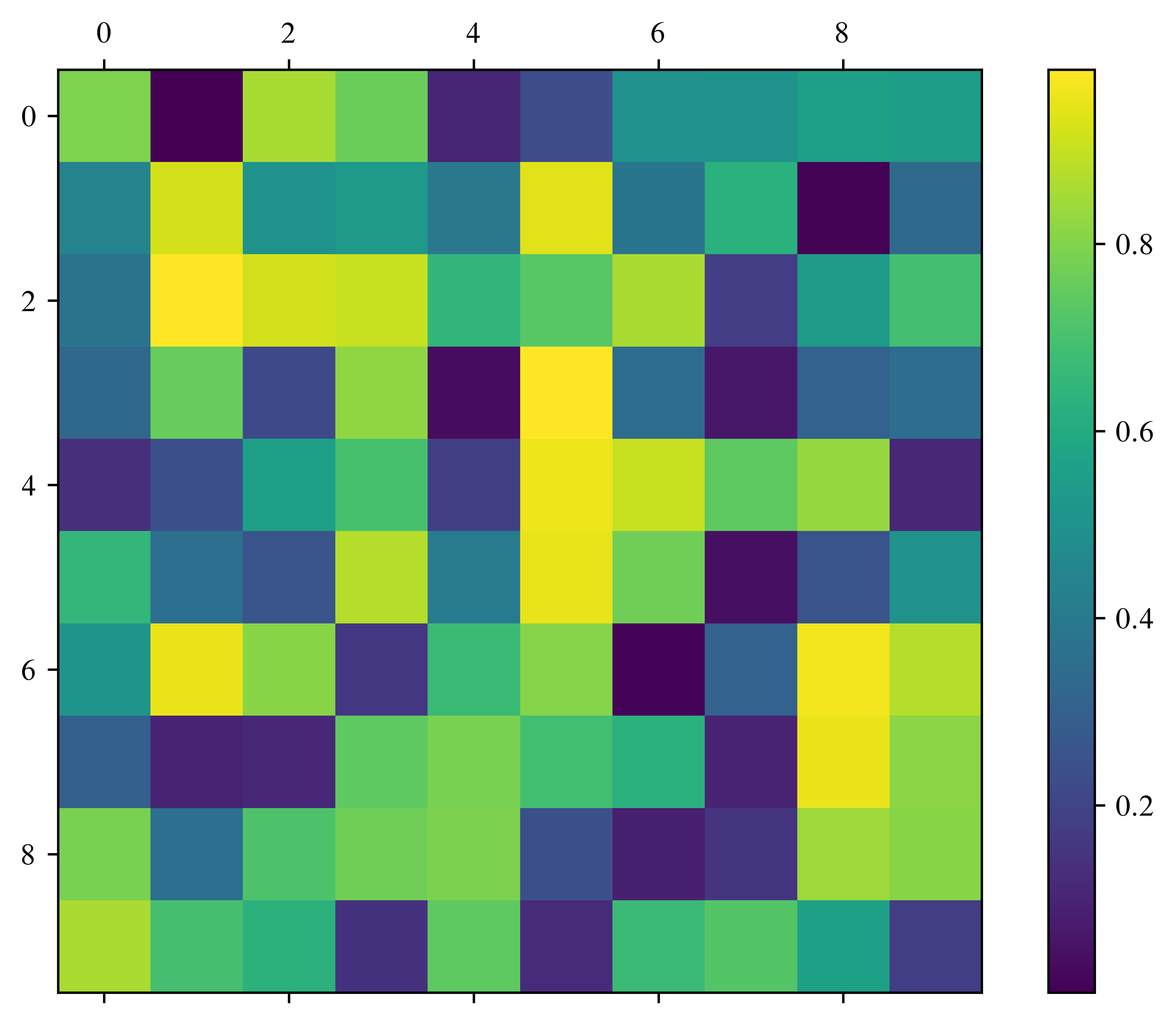
Create a random 10 by 10 matrix
plot the matrix
print the position and the maximal value (argmax)
Bonus for fast people (Is it before 14:20?)
?np.argmaxSignature: np.argmax(a, axis=None, out=None, *, keepdims=<no value>)
Call signature: np.argmax(*args, **kwargs)
Type: _ArrayFunctionDispatcher
String form: <function argmax at 0x768f65f90b80>
File: /usr/lib/python3.13/site-packages/numpy/_core/fromnumeric.py
Docstring:
Returns the indices of the maximum values along an axis.
Parameters
----------
a : array_like
Input array.
axis : int, optional
By default, the index is into the flattened array, otherwise
along the specified axis.
out : array, optional
If provided, the result will be inserted into this array. It should
be of the appropriate shape and dtype.
keepdims : bool, optional
If this is set to True, the axes which are reduced are left
in the result as dimensions with size one. With this option,
the result will broadcast correctly against the array.
.. versionadded:: 1.22.0
Returns
-------
index_array : ndarray of ints
Array of indices into the array. It has the same shape as ``a.shape``
with the dimension along `axis` removed. If `keepdims` is set to True,
then the size of `axis` will be 1 with the resulting array having same
shape as ``a.shape``.
See Also
--------
ndarray.argmax, argmin
amax : The maximum value along a given axis.
unravel_index : Convert a flat index into an index tuple.
take_along_axis : Apply ``np.expand_dims(index_array, axis)``
from argmax to an array as if by calling max.
Notes
-----
In case of multiple occurrences of the maximum values, the indices
corresponding to the first occurrence are returned.
Examples
--------
>>> import numpy as np
>>> a = np.arange(6).reshape(2,3) + 10
>>> a
array([[10, 11, 12],
[13, 14, 15]])
>>> np.argmax(a)
5
>>> np.argmax(a, axis=0)
array([1, 1, 1])
>>> np.argmax(a, axis=1)
array([2, 2])
Indexes of the maximal elements of a N-dimensional array:
>>> ind = np.unravel_index(np.argmax(a, axis=None), a.shape)
>>> ind
(1, 2)
>>> a[ind]
15
>>> b = np.arange(6)
>>> b[1] = 5
>>> b
array([0, 5, 2, 3, 4, 5])
>>> np.argmax(b) # Only the first occurrence is returned.
1
>>> x = np.array([[4,2,3], [1,0,3]])
>>> index_array = np.argmax(x, axis=-1)
>>> # Same as np.amax(x, axis=-1, keepdims=True)
>>> np.take_along_axis(x, np.expand_dims(index_array, axis=-1), axis=-1)
array([[4],
[3]])
>>> # Same as np.amax(x, axis=-1)
>>> np.take_along_axis(x, np.expand_dims(index_array, axis=-1),
... axis=-1).squeeze(axis=-1)
array([4, 3])
Setting `keepdims` to `True`,
>>> x = np.arange(24).reshape((2, 3, 4))
>>> res = np.argmax(x, axis=1, keepdims=True)
>>> res.shape
(2, 1, 4)
Class docstring:
Class to wrap functions with checks for __array_function__ overrides.
All arguments are required, and can only be passed by position.
Parameters
----------
dispatcher : function or None
The dispatcher function that returns a single sequence-like object
of all arguments relevant. It must have the same signature (except
the default values) as the actual implementation.
If ``None``, this is a ``like=`` dispatcher and the
``_ArrayFunctionDispatcher`` must be called with ``like`` as the
first (additional and positional) argument.
implementation : function
Function that implements the operation on NumPy arrays without
overrides. Arguments passed calling the ``_ArrayFunctionDispatcher``
will be forwarded to this (and the ``dispatcher``) as if using
``*args, **kwargs``.
Attributes
----------
_implementation : function
The original implementation passed in.A = np.random.rand(10, 10)
index = np.unravel_index(A.argmax(), A.shape) # np.argmax(A, axis=True)
print(index)
print(A[index])
fig, ax = plt.subplots()
im = ax.matshow(A)
fig.colorbar(im, ax=ax)
plt.show()(np.int64(2), np.int64(1))
0.9860700744651145
Warning: Matrices modifications
# Case1: Asign an array and modify it afterwards
A = np.eye(5)
B = np.eye(5)
C = A  # No hay que hacer
C[0, 0] = 10
print(A)
# now, we'd like to check the equality of the two matrices
# A == B is bad idea for floating point numbers
# np.abs(A-B) < 1e-10 creates a boolean array ( |a_ij-b_ij| < 1e-10 )
# np.all returns True if all entries are True
print("Case1: A == B?", np.all(np.abs(A - B) < 1e-10))

# Case2: Copy an array
A = np.eye(5)
B = np.eye(5)
C = A.copy()
C[0, 0] = 10
print(A)
print("Case2: A == B?", np.all(np.abs(A - B) < 1e-10))

# Case3: Copy all entries
A = np.eye(5)
B = np.eye(5)
C[:, :] = A[:, :]  # all elements
print(A)
C[0, 0] = 10
print("Case3: A == B?", np.all(np.abs(A - B) < 1e-10))
[[10. 0. 0. 0. 0.]
[ 0. 1. 0. 0. 0.]
[ 0. 0. 1. 0. 0.]
[ 0. 0. 0. 1. 0.]
[ 0. 0. 0. 0. 1.]]
Case1: A == B? False
[[1. 0. 0. 0. 0.]
[0. 1. 0. 0. 0.]
[0. 0. 1. 0. 0.]
[0. 0. 0. 1. 0.]
[0. 0. 0. 0. 1.]]
Case2: A == B? True
[[1. 0. 0. 0. 0.]
[0. 1. 0. 0. 0.]
[0. 0. 1. 0. 0.]
[0. 0. 0. 1. 0.]
[0. 0. 0. 0. 1.]]
Case3: A == B? True
What happens here?!
Explanation:
For integers x=y means: The value of x is copied to y.
For large arrays, this copy may be very expensive. The matrix A is stored somewhere in memory. C=A means: Look at the same piece of memory. If you change C, A is changed too, since both (A and C) looking at the same piece of memory.
To avoid this, A.copy() was introduced. This does a (maybe expensive) copy. Use copies wisely.
For some reason, which are beyond of the scope of this course, C[:, :] = A[:, :] does a copy as well.
def create_id_matrix():
    A = np.eye(5)
    return A


def some_matrix_mod(A):
    A[0, 0] = 10.0
    return A
# Case1: create an array via a function
A = np.eye(5)
B = create_id_matrix()
print("Case1:")
print(" A == B?", np.all(np.abs(A - B) < 1e-10))
# Case2: change an array inside a function
A = np.random.rand(5, 5) # has entries between 0 and 1
B = A.copy()
some_matrix_mod(A)
print("Case2:")
print(" A == B?", np.all(np.abs(A - B) < 1e-10))
# Case3: change the identity inside a function
A = np.eye(5)
B = A.copy()
C = some_matrix_mod(A)
print("Case3:")
print(" A == B?", np.all(np.abs(A - B) < 1e-10))
print(" A == C?", np.all(np.abs(A - C) < 1e-10))Case1:
A == B? True
Case2:
A == B? False
Case3:
A == B? False
A == C? True
Weird, isn’t it?
Take home message: If you pass an array to a function, it will be edit inside. It can be always a source of errors.
Exercise:
Predict the behavior of the following functions:
# a save but slow way
# therefore: please avoid this
def some_matrix_mod2(D):
    E = D.copy()
    E[0, :] = 10
    return E


def some_matrix_mod3(D):
    E = D.copy()
    D[-1, -1] = 3
    return E


def some_matrix_mod4(D):
    E = D[:, :]
    D[0, 0] = 3
    return E
# Your prediction (please modify this):
pred_A_equal_B = [False, False, False]
print(pred_A_equal_B)
pred_returns_equal_A = [False, False, False][False, False, False]
Please execute the cell above with your input. Now, check it:
# Array of functions
mat_mods = [some_matrix_mod2, some_matrix_mod3, some_matrix_mod4]

if not np.any(pred_A_equal_B) and not np.any(pred_returns_equal_A):
    print("Please enter your predictions")
else:
    print(not pred_A_equal_B)
    print(not pred_returns_equal_A)
    # for loop over mat_mods; index i increases in parallel
    for i, func in enumerate(mat_mods):
        A = np.random.rand(5, 5)
        B = A.copy()
        C = func(A)
        # A == B
        is_A_equal_B = np.all(np.abs(A - B) < 1e-10)
        # A == C
        is_result_equal_A = np.all(np.abs(A - C) < 1e-10)
        if (
            is_A_equal_B == pred_A_equal_B[i]
            and is_result_equal_A == pred_returns_equal_A[i]
        ):
            print(func, "correct ")
        else:
            print(
                "please modify the prediction for",
                func,
                " and rerun this and the cell above",
            )
Please enter your predictions
pred_A_equal_B[False, False, False]